Example 1
Note
More examples in the form of Jupyter notebooks can be downloaded from the git repository and are contained in the “example_notebooks” directory.
Usage with D9 (the current default viewer)
If you are on a windows system, DS9 may not be available, so move on to the Ginga specification.
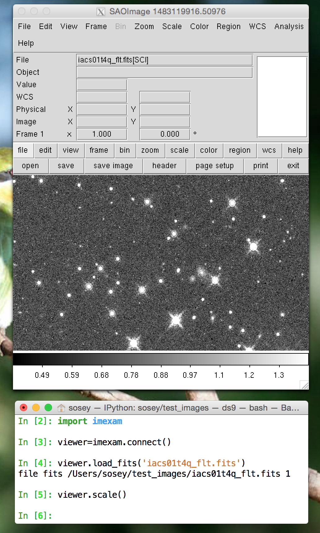
Start up a DS9 window (by default), a new DS9 window will be opened, open a fits image, and scale it:
viewer=imexam.connect()
viewer.load_fits('iacs01t4q_flt.fits')
viewer.scale()
If you already have a window running, you can ask for a list of windows; windows that you start from the imexam package will not show up, this is to keep control over their processes and prevent double assignments.
# This will display if you've used the default command above and have no other DS9 windows open
In [1]: imexam.list_active_ds9()
No active sessions registered
Out[2]: {}

# open a window in another process
In [3]: !ds9&
In [4]: imexam.list_active_ds9()
DS9 ds9 gs /tmp/xpa/DS9_ds9.60457 sosey
Out[5]: {'/tmp/xpa/DS9_ds9.60457': ('ds9', 'sosey', 'DS9', 'gs')}imexam.list_active_ds9()
DS9 ds9 gs 82a7e75f:57222 sosey
You can attach to a current DS9 window be specifying its unique name
viewer1=imexam.connect('ds9')
If you haven’t given your windows unique names using the -t <name> option from the commandline, then you must use the ip:port address:
viewer=imexam.connect('82a7e75f:57222')
Usage with Ginga viewer
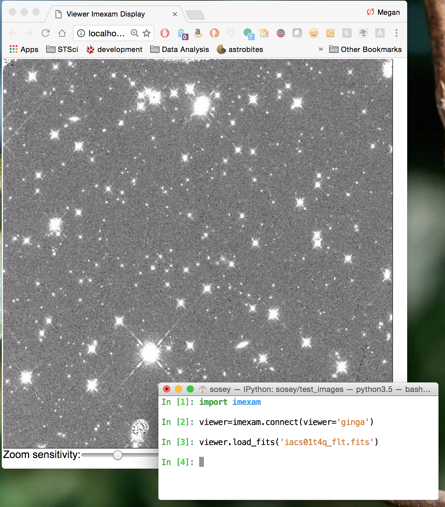
Start up a ginga window using the HTML5 backend and display the same image as above. Make sure that you have installed the most recent version of ginga, imexam will return an error that the viewer cannot be found otherwise.:
viewer=imexam.connect(viewer='ginga')
viewer.load_fits()
Note
All commands after your chosen viewer is opened are the same. Each viewer also has it’s own set of commands which you can additionally use. You may use any viewer for the examples which follow.
Load a fits image into the window:
viewer.load_fits('test.fits')
Scale the image to the default scaling, which is a zscale algorithm, but the viewers other scaling options are also available:
viewer.scale()
viewer.scale('asinh')  <-- uses asinh
Change to heat map colorscheme:
viewer.cmap(color='heat')
Make some marks on the image and save the regions using a DS9 style regions file:
viewer.save_regions('test.reg')
Delete all the regions you made, then load from file:
viewer.load_regions('test.reg')
Plot stuff at the cursor location, in a while loop. Type a key when the mouse is over your desired location and continue plotting with the available options:
viewer.imexam()
Quit out and delete windows and references, for the ginga HTML5 window, this will not close the browser window with the image display, you’ll need to exit that manually. However, if you’ve accidentally closed that window you can reopen and reconnect to the server:
viewer.close()
viewer.reopen()
Example 2
Aperture Photometry
- Perform manual aperture photometry on supplied image
- Make curve of growth and radial profile plots
- Save the profile data and plot to files.
Method 1
Assuming we’ve already connected to the window where the data is displayed:
- This method first uses the “a” key to check out the aperture photometry with the default settings
- Display a radial profile “r” plot around the start we choose
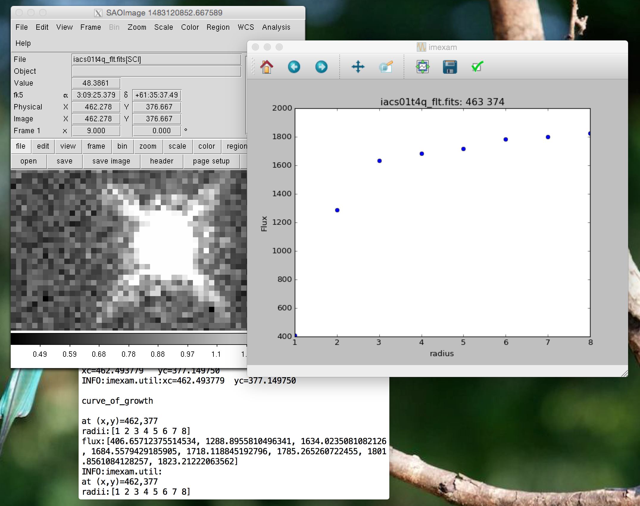
- Look at the curve of growth “g” plot
- Make a new profile plot, print the plotted points to the screen, and save a copy of the plotting window for reference
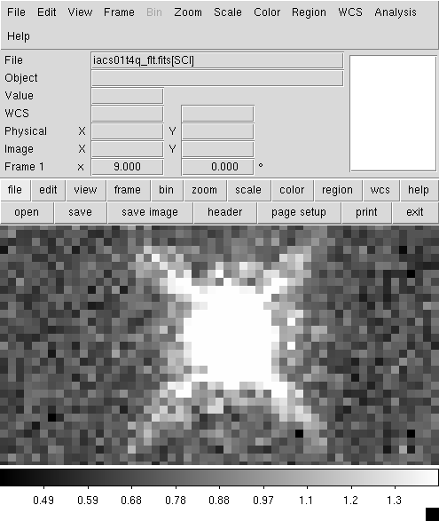
Here a picture of the area I’m looking at on my desktop:
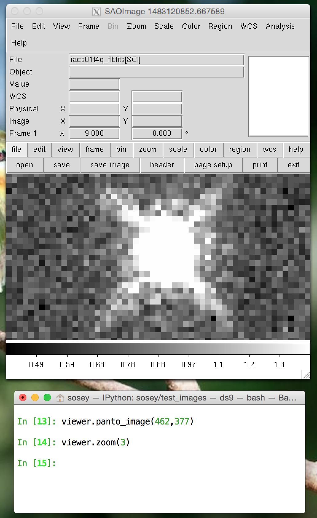
If you wanted to save a screenshot of the viewer display you can use viewer.grab(), in DS9 this will save a snap of the whole DS9 window for reference:
Now let’s start up the imexam() loop and look at a plot of star:
viewer.imexam() #start an imexam session
Use the “r” and “g” keys to look at the radial profile and growth curves:
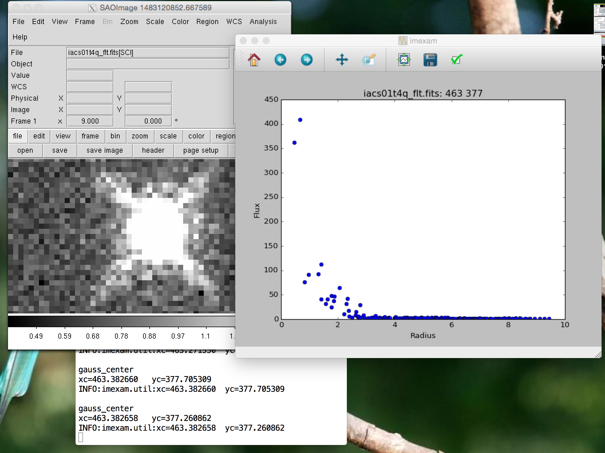
Note that part of the screen information that’s returned includes the flux and radii information:
Let’s take this information and set the radii for our quick aperture photometry:
In [1]: viewer.aimexam()
Out[2]:
{'center': [True, 'Center the object location using a 2d gaussian fit'],
'function': ['aper_phot'],
'radius': [5, 'Radius of aperture for star flux'],
'skyrad': [15, 'Distance to start sky annulus is pixels'],
'subsky': [True, 'Subtract a sky background?'],
'width': [5, 'Width of sky annulus in pixels'],
'zmag': [25.0, 'zeropoint for the magnitude calculation']}

In [3]: viewer.set_plot_pars('a','radius',4)
set aper_phot_pars: radius to 4

In [4]: viewer.set_plot_pars('a','skyrad',8)
set aper_phot_pars: skyrad to 8

In [23]: viewer.imexam()

Press 'q' to quit

2   Make the next plot in a new window
a   Aperture sum, with radius region_size
b   Return the 2D gauss fit center of the object
c   Return column plot
e   Return a contour plot in a region around the cursor
g   Return curve of growth plot
h   Return a histogram in the region around the cursor
j   1D [Gaussian1D default] line fit
k   1D [Gaussian1D default] column fit
l   Return line plot
m   Square region stats, in [region_size],default is median
r   Return the radial profile plot
s   Save current figure to disk as [plot_name]
t   Make a fits image cutout using pointer location
w   Display a surface plot around the cursor location
x   Return x,y,value of pixel
y   Return x,y,value of pixel
Current image /Users/sosey/test_images/iacs01t4q_flt.fits

gauss_center
xc=462.827108       yc=377.705312

aper_phot
x          y        radius    flux       mag(zpt=25.00)  sky    fwhm
462.83     377.71   4         1686.24    16.93           0.92   1.71
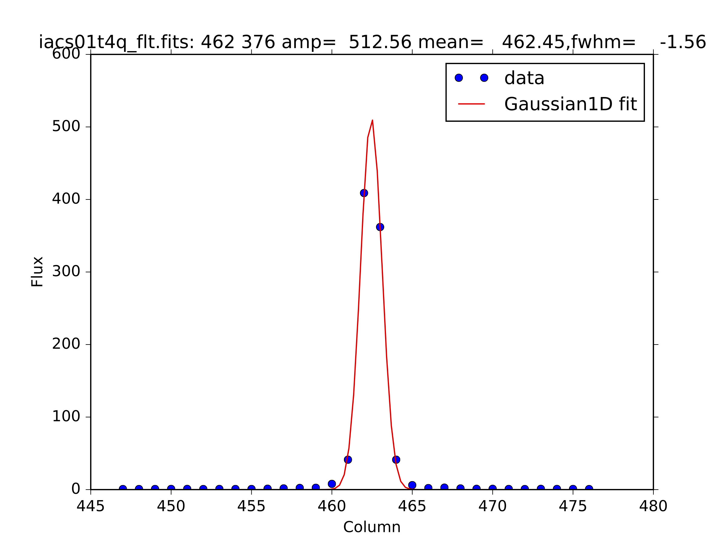
Just for some more information on the star, below is the gaussian fit “j” to the columns of the same star.
Method 2
Assuming we’ve already connected to the DS9 window where the data is displayed:
- First we turn on logging so that everything gets saved to a file
- We then use the “a” key to check out the aperture photometry with the default settings
- Use the “g” to look at the curve of growth
- Adjust the aperture photometry with our our own settings
- We can then use the log file, to create a plot
In [1]: viewer.setlog('mystar.log')
Saving imexam commands to mystar.log
In [2]: viewer.unlearn()

In [3]: viewer.imexam()

Press 'q' to quit

2   Make the next plot in a new window
a   Aperture sum, with radius region_size
b   Return the 2D gauss fit center of the object
c   Return column plot
e   Return a contour plot in a region around the cursor
g   Return curve of growth plot
h   Return a histogram in the region around the cursor
j   1D [Gaussian1D default] line fit
k   1D [Gaussian1D default] column fit
l   Return line plot
m   Square region stats, in [region_size],default is median
r   Return the radial profile plot
s   Save current figure to disk as [plot_name]
t   Make a fits image cutout using pointer location
w   Display a surface plot around the cursor location
x   Return x,y,value of pixel
y   Return x,y,value of pixel
Current image /Users/sosey/test_images/iacs01t4q_flt.fits

xc=462.938220       yc=377.260860
x          y        radius    flux       mag(zpt=25.00)  sky    fwhm
462.94     377.26   5         1739.97    16.90           0.72   1.44

at (x,y)=462,377
radii:[1 2 3 4 5 6 7 8]
flux:[406.65712375514534, 1288.8955810496341, 1634.0235081082126,
1684.5579429185905, 1718.118845192796, 1785.265260722455,
1801.8561084128257, 1823.21222063562]
Lets get some more aperture photometry at larger radii by resetting some of the “a” key values::
In [4]: viewer.set_plot_pars("a","radius",4)
set aper_phot_pars: radius to 4

In [5]: viewer.set_plot_pars("a","skyrad",8)
set aper_phot_pars: skyrad to 8

In [5]: viewer.imexam()  #use the "a" key

xc=463.049330       yc=377.038640
x          y        radius    flux       mag(zpt=25.00)  sky    fwhm
463.05     377.04   4         1679.23    16.94           0.93   1.71
This is what mystar.log contains, you can parse the log, or copy the data and use as you like to make interesting plots later or just have for reference.:
gauss_center
xc=462.938220   yc=377.260860

aper_phot
x          y        radius    flux       mag(zpt=25.00)  sky    fwhm
462.94     377.26   5         1739.97    16.90           0.72   1.44

gauss_center
xc=462.827110   yc=377.371969

gauss_center
xc=462.827109   yc=377.260860

gauss_center
xc=462.827109   yc=377.260860

curve_of_growth

at (x,y)=462,377
radii:[1 2 3 4 5 6 7 8]
flux:[406.65712375514534, 1288.8955810496341, 1634.0235081082126,
1684.5579429185905, 1718.118845192796, 1785.265260722455,
1801.8561084128257, 1823.21222063562]

gauss_center
xc=463.049330   yc=377.038640

aper_phot
x          y        radius    flux       mag(zpt=25.00)  sky    fwhm
463.05     377.04   4         1679.23    16.94           0.93   1.71
Example 3
Advanced Usage - Interact with Daophot and Astropy
While the original intent for the imexam module was to replicate the realtime interaction of the old IRAF imexamine interface with data, there are other possibilities for data analysis which this module can support.One such example, performing more advanced interaction which can be scripted, is outlined below, using familiar IRAF tasks.
Note
You can see a similar photometry example which uses photutils and it’s implementation of DAOPhot aperture photometry instead of IRAF in the imexam_ds9_photometry example jupyter notebook.
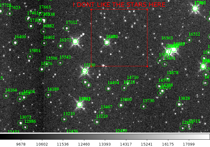
If you have a list of source identifications, perhaps prepared by SExtractor, DAOFind, Starfind or a similar program, you can use imexam to display the science image and overlay apertures for all their locations. From there you can do some visual examination and cleaning up of the list with a combination of region manipulation and useful imexam methods.
Here’s our example image to work with, which is a subsection of a larger image:
I’ll use the IRAF DAOFind to find objects in my field:
from pyraf import iraf
from iraf import noao,digiphot,daophot
from astropy.io import fits

image='iabf01bzq_flt.fits'

fits.info('iabf01bzq_flt.fits')

    Filename: iabf01bzq_flt.fits
    No.    Name         Type      Cards   Dimensions   Format
    0    PRIMARY     PrimaryHDU     210   ()           int16
    1    SCI         ImageHDU        81   (1014, 1014)   float32
    2    ERR         ImageHDU        43   (1014, 1014)   float32
    3    DQ          ImageHDU        35   (1014, 1014)   int16
    4    SAMP        ImageHDU        30   ()           int16
    5    TIME        ImageHDU        30   ()           float32


#set up some finding parameters, you can make this more explicit
iraf.daophot.findpars.threshold=3.0 #3sigma detections only
iraf.daophot.findpars.nsigma=1.5 #width of convolution kernal in sigma
iraf.daophot.findpars.ratio=1.0 #ratio of gaussian axes
iraf.daophot.findpars.theta=0.
iraf.daophot.findpars.sharplo=0.2 #lower bound on feature
iraf.daophot.findpars.sharphi=1.0 #upper bound on feature
iraf.daophot.findpars.roundlo=-1.0 #lower bound on roundness
iraf.daophot.findpars.roundhi=1.0 #upper bound on roundness
iraf.daophot.findpars.mkdetections="no"

    In [84]: iraf.lpar(iraf.daophot.datapars)
           (scale = 1.0)            Image scale in units per pixel
         (fwhmpsf = 2.5)            FWHM of the PSF in scale units
        (emission = yes)            Features are positive?
           (sigma = 1.0)            Standard deviation of background in counts
         (datamin = 0.0)            Minimum good data value
         (datamax = INDEF)          Maximum good data value
           (noise = "poisson")      Noise model
         (ccdread = "")             CCD readout noise image header keyword
            (gain = "ccdgain")      CCD gain image header keyword
       (readnoise = 2.0)            CCD readout noise in electrons
           (epadu = 1.0)            Gain in electrons per count
        (exposure = "exptime")      Exposure time image header keyword
         (airmass = "")             Airmass image header keyword
          (filter = "")             Filter image header keyword
         (obstime = "")             Time of observation image header keyword
           (itime = 1.0)            Exposure time
        (xairmass = INDEF)          Airmass
         (ifilter = "INDEF")        Filter
           (otime = "INDEF")        Time of observation
            (mode = "ql")

iraf.daophot.datapars.datamin=0.
iraf.daophot.datapars.gain="ccdgain"
iraf.daophot.datapars.exposure="exptime"
iraf.daophot.datapars.sigma=105.


#assume the science extension and find some stars
sci="[SCI,1]"
output_locations='iabf01bzq_stars.dat'
iraf.daofind(image=image+sci,output=output_locations,interactive="no",verify="no",verbose="no")

#This is just the top of the file that daofind produced:

    In [24]: more iabf01bzq_stars.dat
    #K IRAF       = NOAO/IRAFV2.16          version    %-23s
    #K USER       = sosey                   name       %-23s
    #K HOST       = intimachay.stsci.edu    computer   %-23s
    #K DATE       = 2014-03-28              yyyy-mm-dd %-23s
    #K TIME       = 15:34:56                hh:mm:ss   %-23s
    #K PACKAGE    = apphot                  name       %-23s
    #K TASK       = daofind                 name       %-23s
    #
    #K SCALE      = 1.                      units      %-23.7g
    #K FWHMPSF    = 2.5                     scaleunit  %-23.7g
    #K EMISSION   = yes                     switch     %-23b
    #K DATAMIN    = 0.                      counts     %-23.7g
    #K DATAMAX    = INDEF                   counts     %-23.7g
    #K EXPOSURE   = exptime                 keyword    %-23s
    #K AIRMASS    = ""                      keyword    %-23s
    #K FILTER     = ""                      keyword    %-23s
    #K OBSTIME    = ""                      keyword    %-23s
    #
    #K NOISE      = poisson                 model      %-23s
    #K SIGMA      = 105.                    counts     %-23.7g
    #K GAIN       = ccdgain                 keyword    %-23s
    #K EPADU      = 2.5                     e-/adu     %-23.7g
    #K CCDREAD    = ""                      keyword    %-23s
    #K READNOISE  = 0.                      e-         %-23.7g
    #
    #K IMAGE      = iabf01bzq_flt.fits[SCI, imagename  %-23s
    #K FWHMPSF    = 2.5                     scaleunit  %-23.7g
    #K THRESHOLD  = 3.                      sigma      %-23.7g
    #K NSIGMA     = 2.                      sigma      %-23.7g
    #K RATIO      = 1.                      number     %-23.7g
    #K THETA      = 0.                      degrees    %-23.7g
    #
    #K SHARPLO    = 0.2                     number     %-23.7g
    #K SHARPHI    = 1.                      number     %-23.7g
    #K ROUNDLO    = -1.                     number     %-23.7g
    #K ROUNDHI    = 1.                      number     %-23.7g
    #
    #N XCENTER   YCENTER   MAG      SHARPNESS   SROUND      GROUND      ID         \
    #U pixels    pixels    #        #           #           #           #          \
    #F %-13.3f   %-10.3f   %-9.3f   %-12.3f     %-12.3f     %-12.3f     %-6d       \
    #
       194.694   2.357     -3.335   0.919       0.141       -0.004      1
       232.659   2.889     -1.208   0.768       0.572       -0.289      2
       237.782   2.925     -1.182   0.669       0.789       -0.971      3
       265.715   2.797     -1.395   0.976       -0.450      -0.669      4
       419.792   2.902     -3.045   0.925       -0.990      0.213       5
       424.566   3.081     -1.202   0.923       0.513       -0.555      6
       534.758   2.856     -1.341   0.659       -0.676      -0.302      7
       580.964   2.485     -1.326   0.821       -0.489      -0.752      8
       587.521   3.568     -1.282   0.911       -0.537      -0.119      9
       725.016   3.999     -1.103   0.714       -0.653      -0.490      10
       736.495   2.808     -1.345   0.710       -0.996      -0.730      11
       746.529   3.200     -0.868   0.303       -0.376      -0.682      12
       757.672   3.172     -1.527   0.420       0.271       0.211       13
       768.768   2.830     -1.321   0.741       -0.842      -0.252      14
       799.199   2.696     -2.096   0.926       0.476       -0.511      15
       807.575   2.445     -4.136   0.745       0.171       -0.131      16
       836.661   2.790     -1.482   0.709       0.205       0.636       17
       879.390   3.069     -1.018   0.549       -0.479      -0.495      18
       912.820   2.806     -1.414   0.576       0.504       0.109       19
       938.794   3.448     -1.731   0.997       -0.239      0.100       20
       17.713    2.731     -1.896   0.286       -0.947      -0.359      21
       48.757    2.755     -1.172   0.586       0.646       -0.543      22
       105.894   3.030     -1.700   0.321       -0.233      -0.006      23
Now we want to read in the file that Daofind produced and save the x,y and ID information. I’m going to read the results using astropy.io.ascii
reader=ascii.Daophot()
photfile=reader.read(output_locations)

#some quick information on what we have now
photfile.colnames

    ['XCENTER', 'YCENTER', 'MAG', 'SHARPNESS', 'SROUND', 'GROUND', 'ID']

photfile.print()

    In [103]: photfile.pprint()
       XCENTER     YCENTER      MAG     SHARPNESS      SROUND       GROUND      ID
    ------------- ---------- --------- ------------ ------------ ------------ ------
    194.694       2.357      -3.335    0.919        0.141        -0.004       1
    232.659       2.889      -1.208    0.768        0.572        -0.289       2
    237.782       2.925      -1.182    0.669        0.789        -0.971       3
    265.715       2.797      -1.395    0.976        -0.450       -0.669       4
    419.792       2.902      -3.045    0.925        -0.990       0.213        5
    424.566       3.081      -1.202    0.923        0.513        -0.555       6
    534.758       2.856      -1.341    0.659        -0.676       -0.302       7
    580.964       2.485      -1.326    0.821        -0.489       -0.752       8
    587.521       3.568      -1.282    0.911        -0.537       -0.119       9
    725.016       3.999      -1.103    0.714        -0.653       -0.490       10
    736.495       2.808      -1.345    0.710        -0.996       -0.730       11
    746.529       3.200      -0.868    0.303        -0.376       -0.682       12
    757.672       3.172      -1.527    0.420        0.271        0.211        13
    768.768       2.830      -1.321    0.741        -0.842       -0.252       14
    799.199       2.696      -2.096    0.926        0.476        -0.511       15
    807.575       2.445      -4.136    0.745        0.171        -0.131       16
You can even pop this up in your web browser if that’s a good format for you: photfile.show_in_browser(). imexam has several functions to help display regions on the DS9 window. Since we have this data loaded into memory, the one we will use here is mark_region_from_array().
Let’s make an array that the method will accept, namely a list of tuples which contain the (x,y,comment) that we want marked to the display. It will also accept any iterator containing a tuple of (x,y,comment).
#lets make a list of our locations as a tuple of x,y,comment
#we'll cut the list to a smaller area and only include those points whose mag is < -4.
locations=list()
for point in range(0,len(photfile['XCENTER']),1):
    if photfile['MAG'][point] < -4:
        locations.append((photfile['XCENTER'][point],photfile['YCENTER'][point],photfile['ID'][point]))

#so the first item looks like:
In [91]: locations[0]
Out[91]: (807.57500000000005, 2.4449999999999998, 16)
Let’s open up a DS9 window (if you haven’t already) and display your image. This will let us display our source locations and play with them
viewer=imexam.connect()
viewer.load_fits('iabf01bzq_flt.fits')
viewer.scale() #scale to DS9 zscale by default
viewer.mark_region_from_array(locations)
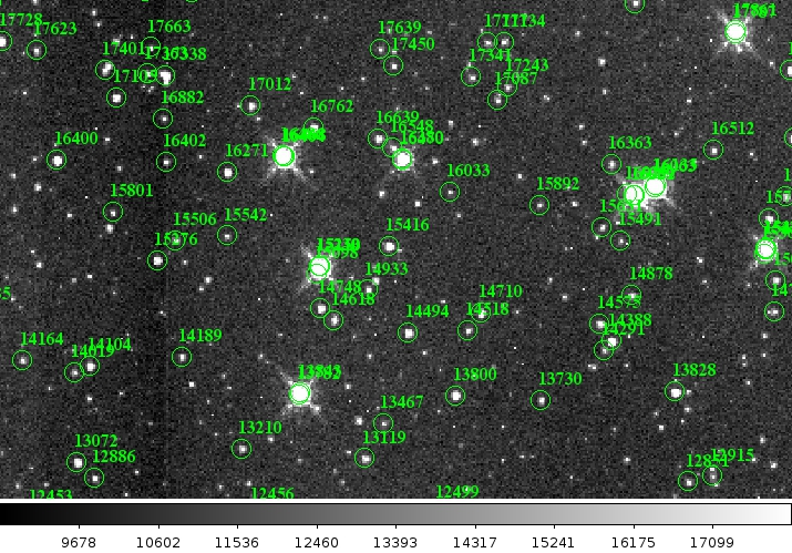
Now we can get rid of some of the stars by hand and save a new file of locations we like. I did this arbitrarily because I decided I didn’t like stars in this part of space. Click on the regions you don’t want and delete them from the screen. You can even add more regions of your own choosing.
You can save these new regions to a DS9 style region file, either through DS9 or imexam
viewer.save_regions('badstars.reg')
Note
A future version of the imexam package will make use of the region interpreter currently being developed with astropy for smoother creation and use of parsable regions files
Here is what the saved region file looks like, you can choose to import this file into any future DS9 display of the same image using the viewer.load_regions() method. You might also want to parse the file to save just the location and comment information in a separate text file.
In [7]: !head badstars.reg
# Region file format: DS9 version 4.1
# Filename: /Users/sosey/ssb/sosey/testme/iabf01bzq_flt.fits[SCI]
global color=green dashlist=8 3 width=1 font="helvetica 10 normal roman" select=1 highlite=1 dash=0 fixed=0 edit=1 move=1 delete=1 include=1 source=1
fk5
circle(0:22:38.709,-72:02:50.58,0.677464")
# text(0:22:39.097,-72:02:50.86) font="time 12 bold" text={ 16 }
circle(0:22:36.340,-72:02:58.27,0.677464")
# text(0:22:36.729,-72:02:58.55) font="time 12 bold" text={ 140 }
circle(0:22:29.068,-72:03:20.78,0.677464")
# text(0:22:29.457,-72:03:21.06) font="time 12 bold" text={ 225 }

            . . .

# text(0:22:56.855,-72:04:23.16) font="time 12 bold" text={ 21985 }
circle(0:22:42.791,-72:05:04.04,0.677464")
# text(0:22:43.180,-72:05:04.32) font="time 12 bold" text={ 22002 }
box(0:22:45.694,-72:04:19.19,14.593",13.1774",149.933) # color=red font="helvetica 16 normal roman" text={I DONT LIKE THE STARS HERE}
Advanced Usage II - Cycle through objects from a list
This example will step through a list of object locations and center that object in the DS9 window with a narrow zoom so that you can examine it further (think about PSF profile creation options here..)
If you haven’t already, start DS9 and load your image into the viewer. I’ll assume that you started DS9 outside of imexam and will need to connect to the window first.
import imexam
imexam.list_active_ds9()

    DS9 1396283378.28 gs 82a7e75f:53892 sosey

viewer=imexam.connect('82a7e75f:53892')

#A little unsure this is the correct window? Let's check by asking what image is loaded. The image I'm working with is iabf01bzq_flt.fits

viewer.get_data_filename()

    '/Users/sosey/ssb/sosey/testme/iabf01bzq_flt.fits'  <-- notice it returned the full pathname to the file

viewer.zoomtofit()  <-- let's zoom out  to see the whole image, incase just a small section was loaded
Read in your list of object locations, I’ll use the same DAOphot targets from the previous example
from astropy.io import ascii
reader=ascii.Daophot()
output_locations='iabf01bzq_stars.dat'
photfile=reader.read(output_locations)

#make some cuts on the list

locations=list()
for point in range(0,len(photfile['XCENTER']),1):
    if photfile['MAG'][point] < -4:
        locations.append((photfile['XCENTER'][point],photfile['YCENTER'][point],photfile['ID'][point])) <-- appending tuple to the list
Take your list of locations and cycle through each one, displaying a zoomed in section on the DS9 window and starting imexam for each coordinate. I’m just going to go through 10 or so random stars. You can set this up however you like, including using a keystroke as your stopping condition in conjunction with viewer.readcursor()
I’ll also mark the object we’re interested in on the display for reference
viewer.zoom(8)
for object in locations[100:110]:
    viewer.panto_image(object[0],object[1])
    viewer.mark_region_from_array(object)
    viewer.imexam()
Example 4
Load and examine an image CUBE
Note
image cubes are currently only supported for the DS9 viewer.
Image cubes can be multi-extension fits files which have multidimensional (> 2) images in any of their extensions. When they are loaded into DS9, a cube dialog frame is opened along with a box which allows the user to control which slices are displayed. Here’s what the structure of such a file might look like:
astropy.io.fits.info('test_cube.fits')

Filename: test_cube.fits
No.    Name         Type      Cards   Dimensions   Format
0    PRIMARY     PrimaryHDU     215   ()
1    SCI         ImageHDU        13   (1032, 1024, 35, 5)   int16
2    REFOUT      ImageHDU        13   (258, 1024, 35, 5)   int16
You can use all the regular imexam methods with this image, including imexam() and the current slice which you have selected will be used for analysis. You can also ask imexam which slice is display, or the full image information of what is in the current frame for your own use (ds9 is just the name I chose, you can call the control object connected to your display window anything)
viewer=imexam.connect()
viewer.load_fits('test_cube.fits')
viewer.window.get_filename()

Out[24]: '/Users/sosey/ssb/imexam/test_cube.fits'

viewer.window.get_frame_info()
Out[25]: '/Users/sosey/ssb/imexam/test_cube.fits[SCI,1](0, 0)'
Now I’m going to use the Cube dialog to change the slice I’m looking at to (4,14) -> as displayed in the dialog. DS9 displayed 1-indexed numbers, and the fits utitlity behind imexam uses 0-indexed numbers, so expect the return to be off by a value of 1.
Let’s ask for the information again:
In [26]: viewer.window.get_filename()
Out[26]: '/Users/sosey/ssb/imexam/test_cube.fits'

In [27]: viewer.window.get_frame_info()
Out[27]: '/Users/sosey/ssb/imexam/test_cube.fits[SCI,1](3, 13)'
You can ask for just the information about which slice is displayed and it will return the tuple(extension n, ...., extension n-1). The extensions are ordered in row-major form in astropy.io.fits:
In [28]: viewer.window.get_slice_info()
Out[28]: (3, 13)
The returned tuple contains just which 2d slice is displayed. In our cube image, which is 4D (1032, 1024, 35, 5) == (NAXIS1, NAXIS2, NAXIS3, NAXIS4) in DS9, however in astropy.io.fits this is (5,35,1024,1032) == (NAXIS4, NAXIS3, NAXIS2, NAXIS1)
By default, the first extension will be loaded from the cube fits file if none is specified. If you would rather see another extension, you can load it the same as with simpler fits files:
viewer.load_fits('test_cube.fits',extname='REFOUT')
Example 5
Use the imexamine library standalone to create plots without viewing
It’s possible to use the imexamine library of plotting functions without loading an image into the viewer. All of the functions take 3 inputs: the x, y, and data array. In order to access the function, first create an imexamine object:
from imexam.imexamine import Imexamine
import numpy as np

data=np.random.rand((100,100)) #create a random array thats 100x100 pixels
plots=Imexamine()
These are the functions you now have access to:
plots.aper_phot                 plots.contour_plot              plots.histogram_plot            plots.plot_line                 plots.set_colplot_pars          plots.set_surface_pars
plots.aperphot_def_pars         plots.curve_of_growth_def_pars  plots.imexam_option_funcs       plots.plot_name                 plots.set_column_fit_pars       plots.show_xy_coords
plots.aperphot_pars             plots.curve_of_growth_pars      plots.line_fit                  plots.print_options             plots.set_contour_pars          plots.showplt
plots.colplot_def_pars          plots.curve_of_growth_plot      plots.line_fit_def_pars         plots.register                  plots.set_data                  plots.sleep_time
plots.colplot_pars              plots.do_option                 plots.line_fit_pars             plots.report_stat               plots.set_histogram_pars        plots.surface_def_pars
plots.column_fit                plots.gauss_center              plots.lineplot_def_pars         plots.report_stat_def_pars      plots.set_line_fit_pars         plots.surface_pars
plots.column_fit_def_pars       plots.get_options               plots.lineplot_pars             plots.report_stat_pars          plots.set_lineplot_pars         plots.surface_plot
plots.column_fit_pars           plots.get_plot_name             plots.new_plot_window           plots.reset_defpars             plots.set_option_funcs          plots.unlearn_all
plots.contour_def_pars          plots.histogram_def_pars        plots.option_descrip            plots.save_figure               plots.set_plot_name
plots.contour_pars              plots.histogram_pars            plots.plot_column               plots.set_aperphot_pars         plots.set_radial_pars
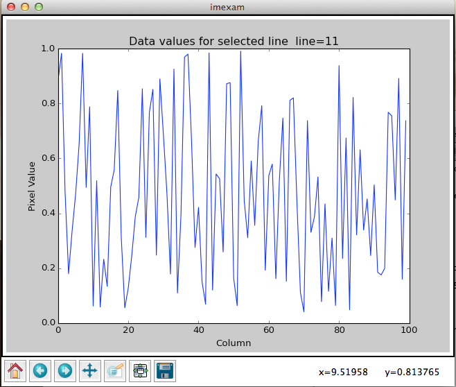
To create a plot, just specify the method:
plots.plot_line(10,10,data)
produces the following plot:
You can then save the current plot using the save method:
plots.contour(10,10,data)
plots.save() # with an optional filename using filename="something.extname"

In [1]: plots.plot_name
Out[2]: 'imexam.pdf'

plots.close() # close the plot window
Where the extname specifies the format of the file, ex: jpg or pdf. A pdf file will be the default output, using the curent self.plot_name.
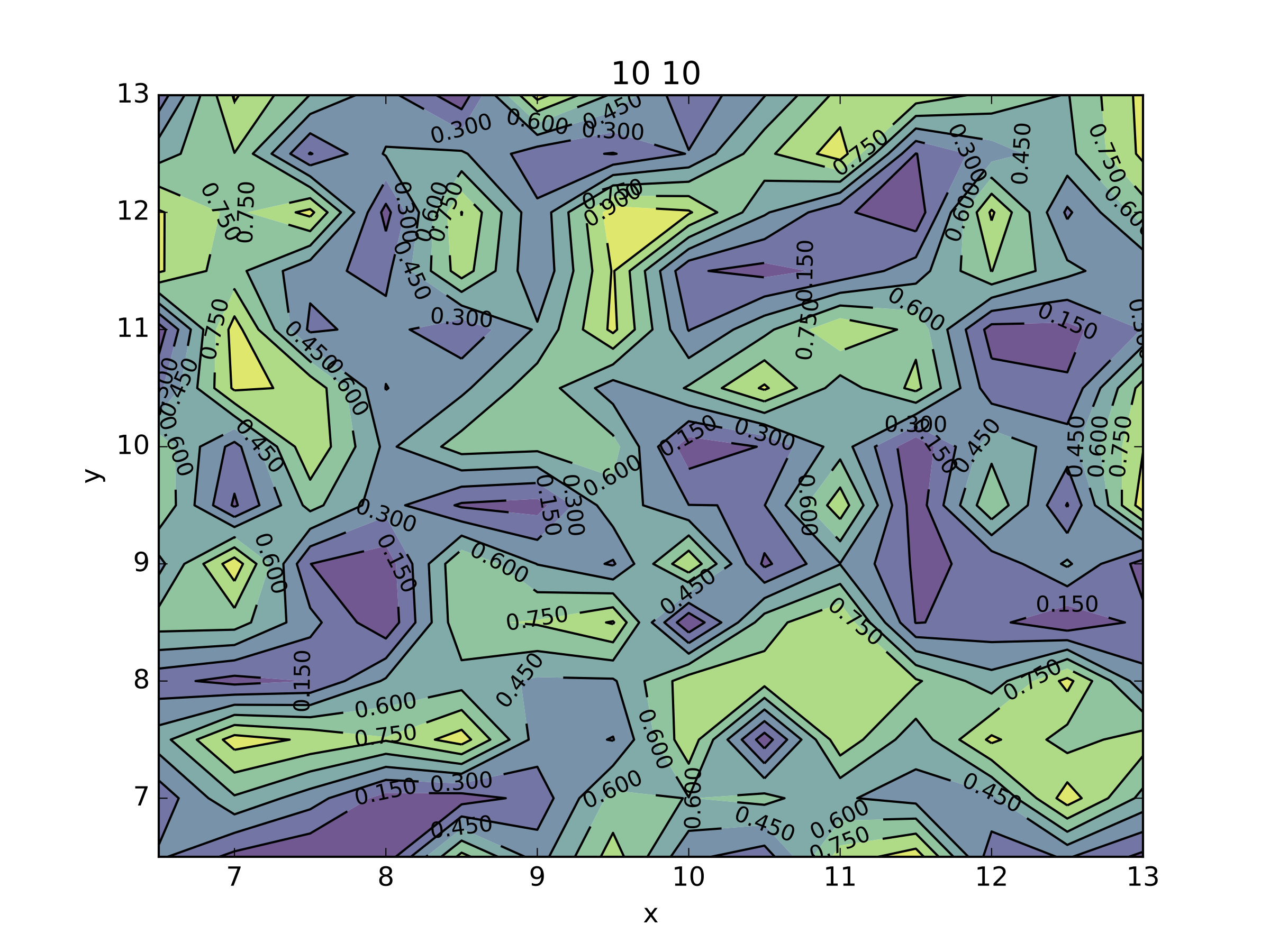
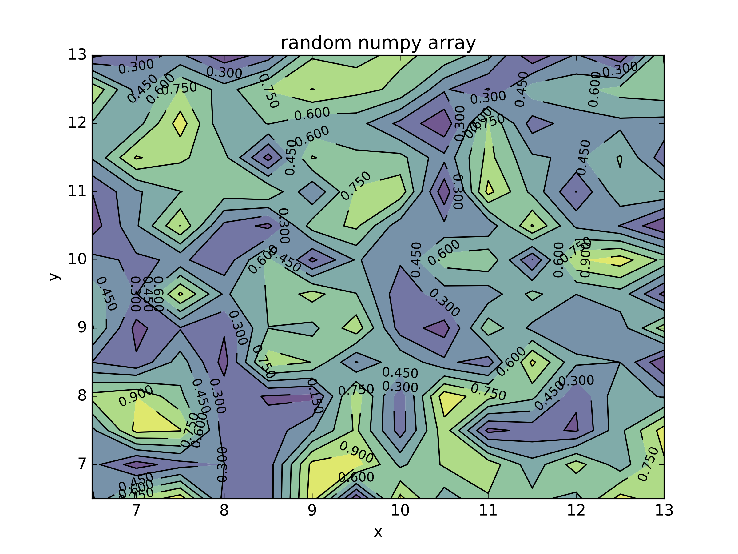
Note that no name is attached to the above contour plot because we plotted a data array. When you are using the plotting class without a viewer, you can attach any title you like by editing the plotting parameters using the dictionary directly::
plots.contour_pars['title'][0] = "random numpy array"
Return information to variables without plotting
Some of the imexamine() methods are capable of returning their results as data objects. First, lets import some useful things to use in the examples:
from astropy.io import fits
from imexam.imexamine import Imexamine

# get my example data from a fits image
data=fits.getdata()
Return the fitting result for a line (the same can be done for column_fit):
In [1]: plots.line_fit(462, 377, data, genplot=False)
using model: <class 'astropy.modeling.functional_models.Gaussian1D'>
Name: Gaussian1D
Inputs: ('x',)
Outputs: ('y',)
Fittable parameters: ('amplitude', 'mean', 'stddev')
xc=462.438219       yc=377.038640
Out[1]: <Gaussian1D(amplitude=512.5638896303021, mean=462.45102207881393, stddev=-0.6638566150545719)>

# I could have specified an output object here instead and saved the model object:

In [1]: results = plots.line_fit(462, 377, data, genplot=False)
using model: <class 'astropy.modeling.functional_models.Gaussian1D'>
Name: Gaussian1D
Inputs: ('x',)
Outputs: ('y',)
Fittable parameters: ('amplitude', 'mean', 'stddev')
xc=462.438219       yc=377.038640

In [2]: results
Out[2]: <Gaussian1D(amplitude=512.5638896303021, mean=462.45102207881393, stddev=-0.6638566150545719)>

In [3]: type(results)
Out[3]:
<class 'astropy.modeling.functional_models.Gaussian1D'>
Name: Gaussian1D
Inputs: ('x',)
Outputs: ('y',)
Fittable parameters: ('amplitude', 'mean', 'stddev')
Return the radial profile data points:
In [1]: results = plots.radial_profile(462, 377, data, genplot=False)
xc=462.438220       yc=377.038640

# here, results is a tuple of the radius and the flux arrays
In [2]: type(results)
Out[2]: tuple

In [3]: results
Out[3]:
(array([ 0.43991986,  0.56310764,  1.05652729,  1.11346785,  1.12730166,
         1.18083435,  1.4387386 ,  1.56225828,  1.72993907,  1.77404857,
         1.83394967,  1.8756147 ,  2.00971898,  2.0402282 ,  2.08520709,
         2.11462747,  2.43216151,  2.43852579,  2.49490037,  2.50720797,
         2.56207175,  2.56811411,  2.62090222,  2.65022406,  2.73622589,
         2.76432473,  2.99360832,  3.0141751 ,  3.07007625,  3.09013412,
         3.12919301,  3.17820187,  3.22639932,  3.27395339,  3.29213154,
         3.34795643,  3.36181609,  3.41650254,  3.43843675,  3.56198995,
         3.57009352,  3.59167466,  3.68924014,  3.71012829,  3.83595742,
         3.89592694,  3.91565741,  3.95831886,  3.97442453,  3.98552521,
         3.9971748 ,  4.00099637,  4.0623451 ,  4.06610542,  4.0775248 ,
         4.10394097,  4.21436241,  4.25811375,  4.28708374,  4.33010037,
         4.43838783,  4.53773166,  4.541146  ,  4.55813187,  4.56194401,
         4.58853854,  4.63205502,  4.65159003,  4.66197958,  4.67852677,
         4.68183843,  4.71753044,  4.71757631,  4.78260702,  4.85229095,
         4.88403989,  4.96555878,  4.98067583,  4.99306443,  4.99658806,
         5.05766026,  5.06986075,  5.16561429,  5.20137031,  5.2398823 ,
         5.24535309,  5.27513495,  5.30395753,  5.32716192,  5.33548947,
         5.37876614,  5.3848761 ,  5.43835691,  5.43870338,  5.48116519,
         5.52253984,  5.52811091,  5.53651564,  5.56191459,  5.58370969,
         5.59757142,  5.64425498,  5.65248702,  5.65793014,  5.78110428,
         5.80777797,  5.89748546,  5.92363512,  5.94896363,  5.97744528,
         5.98777194,  6.00070036,  6.03626122,  6.04170629,  6.05451954,
         6.06471496,  6.09265553,  6.09993812,  6.10748513,  6.13239687,
         6.16254603,  6.17042707,  6.19224411,  6.20754751,  6.22957178,
         6.23733343,  6.30103604,  6.33772298,  6.43833558,  6.44070886,
         6.48849245,  6.50959949,  6.51230262,  6.52146032,  6.5595647 ,
         6.56189413,  6.63183044,  6.64347305,  6.65679268,  6.71458743,
         6.72804634,  6.73034962,  6.73980232,  6.75327507,  6.77383526,
         6.79689127,  6.82830694,  6.84864187,  6.87117266,  6.87342797,
         6.8817999 ,  6.94435706,  6.9488506 ,  6.97513961,  6.98399121,
         7.01080949,  7.08663012,  7.10837617,  7.11926989,  7.13440215,
         7.19907049,  7.23120275,  7.3613401 ,  7.37600509,  7.41364442,
         7.41776616,  7.43206628,  7.45308634,  7.49419535,  7.50475127,
         7.50650756,  7.55930201,  7.56802554,  7.60008443,  7.66481157,
         7.70503555,  7.76414132,  7.81964293,  8.06920371,  8.12646314,
         8.12808509,  8.15298819,  8.17548548,  8.20966328,  8.22630274,
         8.25580581,  8.27314042,  8.32288269,  8.77430839,  8.8269951 ,
         8.83372905,  8.86536955,  8.91032754,  8.91751826,  9.48215209,
         9.56647781]),
 array([ 408.87057495,   41.23228073,   91.90717316,   48.38606262,
         112.11755371,   64.6014328 ,  361.9876709 ,    7.88528776,
          76.15605927,   92.4905777 ,    5.74170589,    8.54299355,
          37.25744629,   17.17868423,   41.94879532,   29.16669464,
          25.11438942,   41.24355316,   31.41527748,    2.35880852,
           2.51266503,    3.61639667,   31.96870041,   47.24103928,
           1.86882472,    2.25345397,    3.43679786,    2.95230484,
           7.01711893,    4.25243187,   10.45163536,   15.06377506,
           2.06799817,    1.55962014,    3.2355001 ,    3.58886528,
           4.77823544,    2.61030412,    6.15013599,    2.26734257,
           3.79847336,    5.18475103,    2.02961087,    1.86825836,
           2.26850033,    1.98072493,    2.40412855,    2.35658216,
           2.2638216 ,    1.48555958,    2.15530491,    1.40320516,
           2.42260337,    3.59516048,    1.49309242,    2.70001984,
           1.35936797,    2.50372696,    1.99834633,    2.1075139 ,
           2.10088921,    3.91031456,    1.40116227,    1.58724546,
           1.64244962,    4.27553177,    2.86458731,    2.07594514,
           1.24715221,    1.55571783,    3.28257489,    1.08224833,
           1.99108934,    1.28673184,    2.22391272,    2.01411462,
           1.27933741,    2.57424259,    2.27977562,    1.34119225,
           2.46366167,    2.04145074,    2.27879167,    3.32902098,
           2.0256803 ,    3.04667783,    3.214293  ,    2.71672273,
           1.18290937,    3.39013147,    2.61141396,    1.24552131,
           2.7109127 ,    1.20734   ,    1.065956  ,    2.0110569 ,
           2.63785267,    2.08804011,    1.23607028,    1.53105474,
           2.9585526 ,    0.92856985,    1.70498252,    0.98702717,
           3.00484014,    2.96310997,    1.10799265,    1.02301562,
           2.59040713,    1.55507016,    1.1307373 ,    1.46614468,
           3.7729485 ,    0.8989926 ,    1.81300449,    1.49930847,
           0.97070342,    3.58096623,    1.45315814,    1.37846851,
           1.22037327,    2.02710581,    3.06499743,    1.60018504,
           3.15293145,    1.34511912,    1.04039967,    0.94602752,
           1.5991565 ,    1.11648059,    0.90265507,    1.25119698,
           1.32048595,    1.331002  ,    1.26167858,    0.81102282,
           0.99124312,    0.76625013,    1.42264056,    1.41574192,
           1.67775941,    1.15894651,    1.19685972,    0.99676919,
           1.16761708,    1.20492256,    1.09948123,    1.0989542 ,
           0.92135239,    0.89912277,    1.15777898,    1.07870626,
           1.32945871,    1.06859183,    0.77524334,    1.4281857 ,
           1.05790067,    1.08861005,    1.03711545,    1.00277674,
           1.11795783,    1.04079187,    1.77855933,    0.875655  ,
           1.70616186,    0.95955884,    1.2846061 ,    0.9819802 ,
           1.09096873,    1.12618971,    2.52278042,    1.14947557,
           2.55132389,    1.16845107,    1.0366509 ,    1.03310716,
           0.76811701,    0.98454052,    1.38449657,    1.41319823,
           1.30402267,    1.26531458,    0.88282102,    1.33250594,
           0.86149669,    1.13119161,    0.89653128,    1.47101414,
           2.82045436,    2.37812138,    0.82307637,    1.3075676 ,
           1.45813155,    1.30278611,    1.60565269,    1.01857305], dtype=float32))
Return the curve of growth points:
In [1]: results = plots.curve_of_growth(462, 377, data, genplot=False)
xc=462.438220       yc=377.038640

at (x,y)=462,377
radii:[1 2 3 4 5 6 7 8]
flux:[406.65712375514534, 1288.8955810496341, 1634.0235081082126, 1684.5579429185905, 1718.118845192796, 1785.265260722455, 1801.8561084128257, 1823.21222063562]

In [2]: type(results)
Out[2]: tuple

In [3]: results
Out[3]:
(array([1, 2, 3, 4, 5, 6, 7, 8]),
 [406.65712375514534,
  1288.8955810496341,
  1634.0235081082126,
  1684.5579429185905,
  1718.118845192796,
  1785.265260722455,
  1801.8561084128257,
  1823.21222063562])

 # the typle can be separated into it's parts
 radius, flux = results
Return the histogram information as a tuple of values and bin edges:
In [1]: counts, bins = plots.histogram(462, 377, data, genplot=False)

In [2]: counts
Out[2]:
array([372,   7,   1,   1,   1,   0,   1,   3,   1,   2,   1,   2,   0,
          0,   0,   1,   0,   0,   1,   0,   0,   0,   2,   0,   0,   0,
          0,   1,   0,   0,   0,   0,   0,   0,   0,   0,   0,   0,   0,
          0,   0,   0,   0,   0,   0,   0,   0,   0,   0,   0,   0,   0,
          0,   0,   0,   0,   0,   0,   0,   0,   0,   0,   0,   0,   0,
          0,   0,   0,   0,   0,   0,   0,   0,   0,   0,   0,   0,   0,
          0,   0,   0,   0,   0,   0,   0,   0,   0,   0,   1,   0,   0,
          0,   0,   0,   0,   0,   0,   0,   0,   0]

In [3]: bins
Out [3]:
 array()[   0.58091092,    4.66380756,    8.7467042 ,   12.82960084,
          16.91249748,   20.99539412,   25.07829076,   29.1611874 ,
          33.24408404,   37.32698068,   41.40987732,   45.49277396,
          49.5756706 ,   53.65856725,   57.74146389,   61.82436053,
          65.90725717,   69.99015381,   74.07305045,   78.15594709,
          82.23884373,   86.32174037,   90.40463701,   94.48753365,
          98.57043029,  102.65332693,  106.73622357,  110.81912021,
         114.90201685,  118.98491349,  123.06781013,  127.15070677,
         131.23360341,  135.31650005,  139.39939669,  143.48229333,
         147.56518997,  151.64808661,  155.73098325,  159.81387989,
         163.89677653,  167.97967317,  172.06256981,  176.14546645,
         180.22836309,  184.31125973,  188.39415637,  192.47705302,
         196.55994966,  200.6428463 ,  204.72574294,  208.80863958,
         212.89153622,  216.97443286,  221.0573295 ,  225.14022614,
         229.22312278,  233.30601942,  237.38891606,  241.4718127 ,
         245.55470934,  249.63760598,  253.72050262,  257.80339926,
         261.8862959 ,  265.96919254,  270.05208918,  274.13498582,
         278.21788246,  282.3007791 ,  286.38367574,  290.46657238,
         294.54946902,  298.63236566,  302.7152623 ,  306.79815894,
         310.88105558,  314.96395222,  319.04684886,  323.1297455 ,
         327.21264215,  331.29553879,  335.37843543,  339.46133207,
         343.54422871,  347.62712535,  351.71002199,  355.79291863,
         359.87581527,  363.95871191,  368.04160855,  372.12450519,
         376.20740183,  380.29029847,  384.37319511,  388.45609175,
         392.53898839,  396.62188503,  400.70478167,  404.78767831,
         408.87057495])