Comparison with the IRAF verison of imexamine
The following is a comparison of the outputs, returned values and user options for this module versus imexamine in IRAF
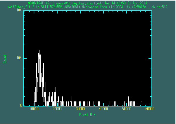
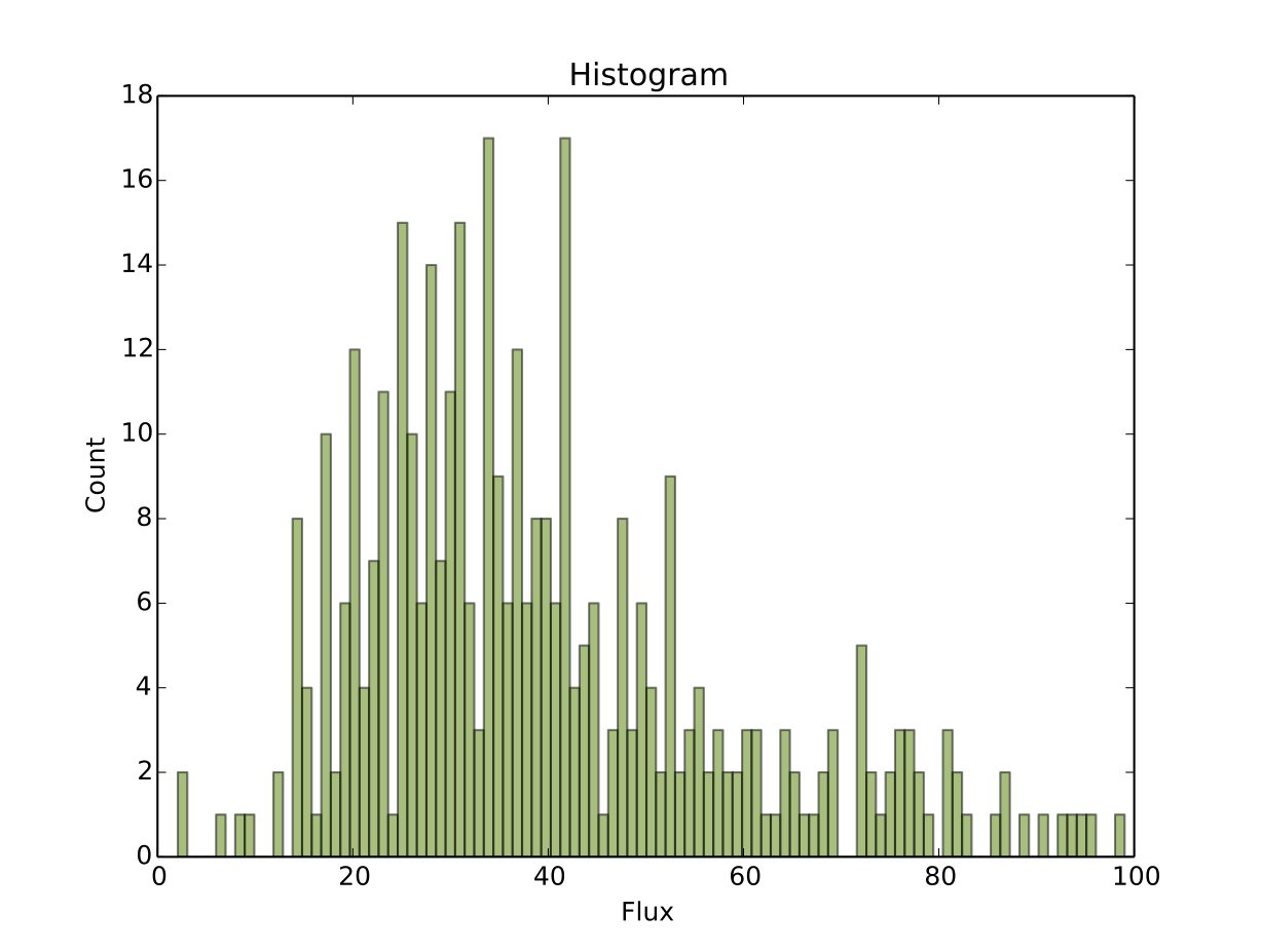
All plot types are replicated between the codes, though they may be rendered differently. The images below are representative of the basic plots from each package.
The same user plot options, as in the rimexam, cimexam etc. type IRAF param files are replicated to their useful extent using python dictionaries for each imexamine key.
Colormaps and point styles for the matplotlib plots may be changed by the user through the
imexamkey default dictionariesIn
imexam, once the plot is displayed on the screen, you can zoom in and out using the controls in the plotting window.imexamallows users to register their own analysis functionsimexamdoes not attempt to replicate the colon command interaction, if users wish to change the plot settings they should exit the imexam() method, reset the options and call it again.all of the imexam() functions in
imexamcan be called by themselves if you supply an x,y coordinate
How do the numerical results compare with the IRAF version? This is a little harder to judge with cursor centering. Visual comparison of the resulting plots shows good agreement, as well as some random checks of the photometry and statistical return methods.
Statistical returns
IRAF “m” key:
- ::
–> imexam
# SECTION NPIX MEAN MEDIAN STDDEV MIN MAX
[584:588,697:701] 25 46533. 51314. 10281. 21215. 56186.
imexam “m” key (with cursor location flooring):
[583:588,695:700] median: 51458.000000
imexam only shows one statistic at a time. The same function call may be used to show the results from any valid numpy function, it will return an attribute error for invalid functions.
For example, if you edit the defaults dictionary for the “m” key:
viewer.mimexam()

    {'function': ['report_stat'],
     'region_size': [5, 'region size in pixels to use'],
     'stat': ['median',
     'which numpy stat to return [median,min,max...must map to a numpy func]']}

viewer.exam.report_stat_pars["stat"][0] = "max"  <---- will report np.max for the array

    [584:589,695:700] amax: 56186.000000

viewer.exam.report_stat_pars["stat"][0] = "mean"  <---- will report np.mean for the array

    [583:588,694:699] mean: 45412.878906

viewer.exam.report_stat_pars["stat"][0]="std"

    [583:588,694:699] std: 10706.179688
Aperture Photometry
IRAF “a” key:
#   COL    LINE   COORDINATES
#     R    MAG    FLUX     SKY    PEAK    E   PA BETA ENCLOSED   MOFFAT DIRECT
585.81  698.16 585.81 698.16
17.51   8.86 2.858E6  10840.  45443. 0.03  -64 8.32     5.23     7.10   5.83
imexam “a” key (using the defaults):
xc=586.138728   yc=697.990516
x       y       radius  flux    mag(zpt=25.00)  sky     fwhm
586.14  697.99  5       1508664.63      9.55    11160.89        6.03
The “xc” and “yc” returns are the gaussian fit centers, as well as the FWHM from the fit. If we set the values to be similar to what IRAF.imexamine used, we can see the numbers are closer, the radius for the apertures are floored though before being sent to photutil:
viewer.aimexam()

{'center': [True, 'Center the object location using a 2d gaussian fit'],
 'function': ['aperphot'],
 'radius': [5, 'Radius of aperture for star flux'],
 'skyrad': [15, 'Distance to start sky annulus is pixels'],
 'subsky': [True, 'Subtract a sky background?'],
 'width': [5, 'Width of sky annulus in pixels'],
 'zmag': [25.0, 'zeropoint for the magnitude calculation']}


viewer.exam.aperphot_pars["radius"][0]=17.5

xc=586.213790   yc=697.501845
x       y       radius  flux    mag(zpt=25.00)  sky     fwhm
586.21  697.50  17      2565167.11      8.98    11162.83        6.02
Radial Profile Plot
The fit profile of the star out to the specified radius.
Users can look at the fit profile of the star using the 1D gaussian option.
By default, imexam prints the data point values to the screen.
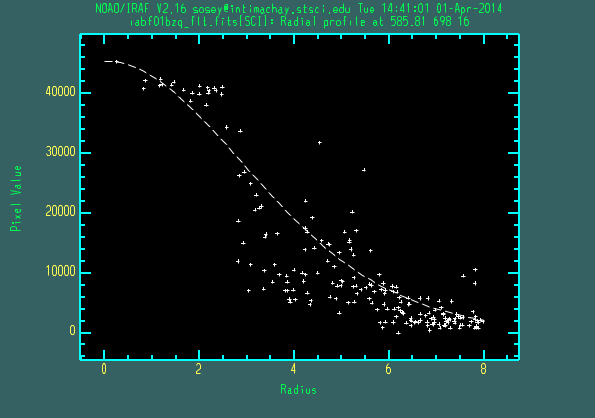
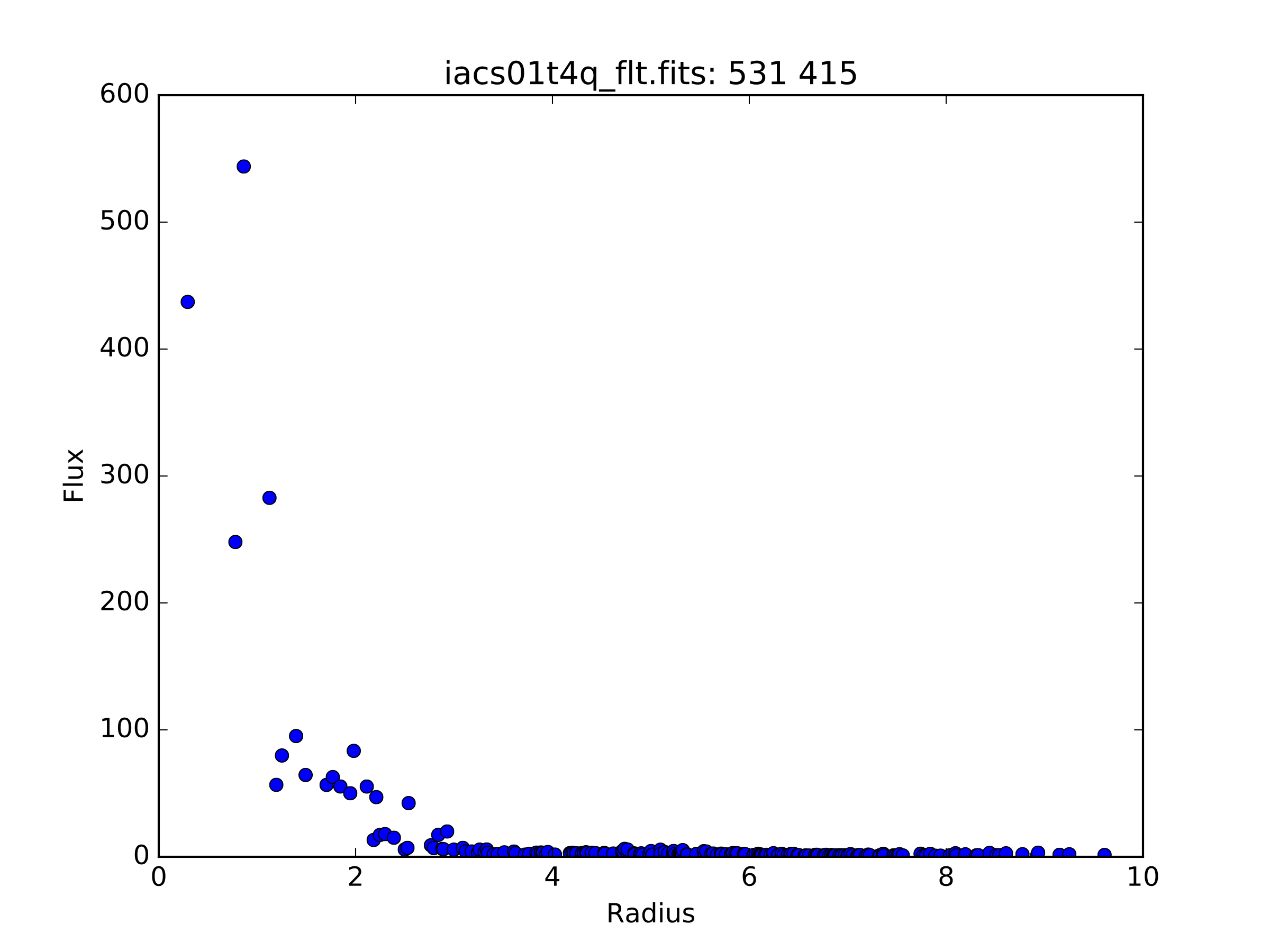
imexam prints the plotted data to the screen
pressed: r
xc=655.659205   yc=698.937124
Sky per pixel: 0.7021602984249302 using(rad=10.0->15.0)

at (x,y)=655,698
radii:[0 1 2 3 4 5 6 7 8 9]
flux:[  74.23025852  153.66757441   60.17693806    9.7988813     7.10537578
    9.08464076    3.1673068     2.92777784    0.26435121    0.18440688]

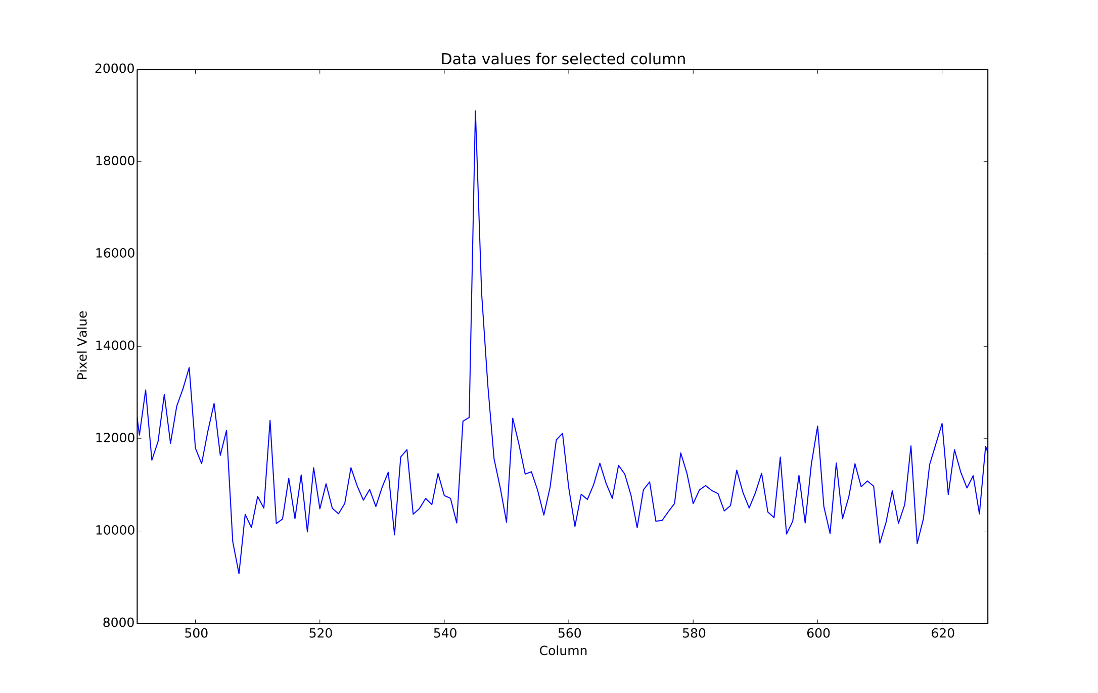
Column and Line plots

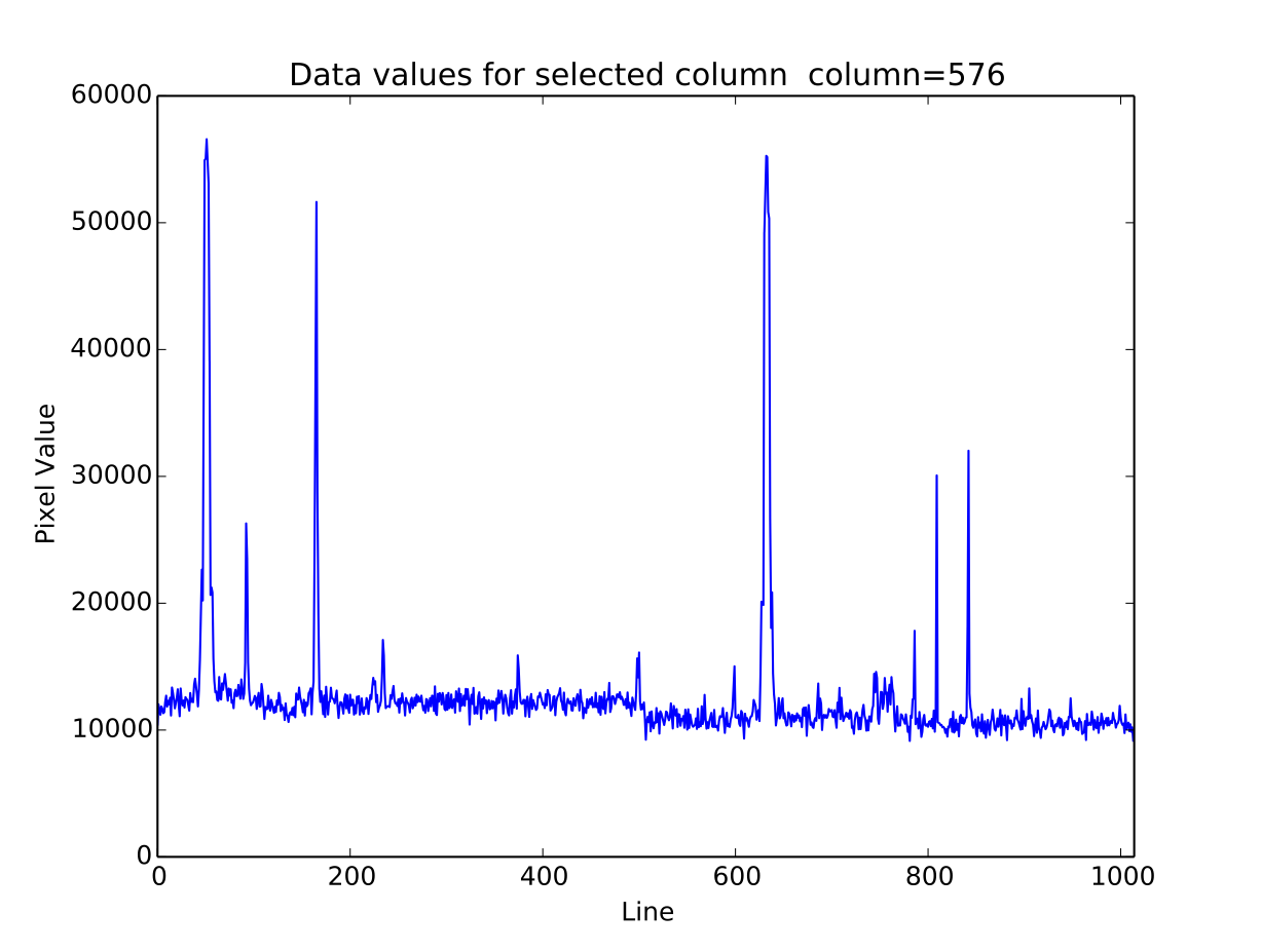
Keep in mind that python is 0-index and IRAF returns 1-index arrays, so the equivalent IRAF plot of 587 is really 588:
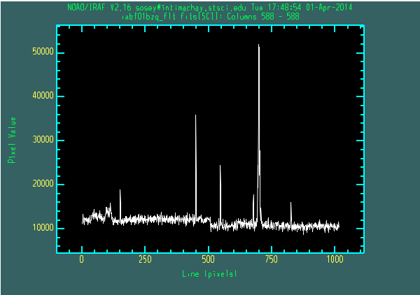
.
An added benefit in the python package is that you can zoom in and out of the plots using the window controls, below is a zoomed in area of the column plot as it appears in the window:
1D Gaussian plots
These plots are representative for both the column and line versions

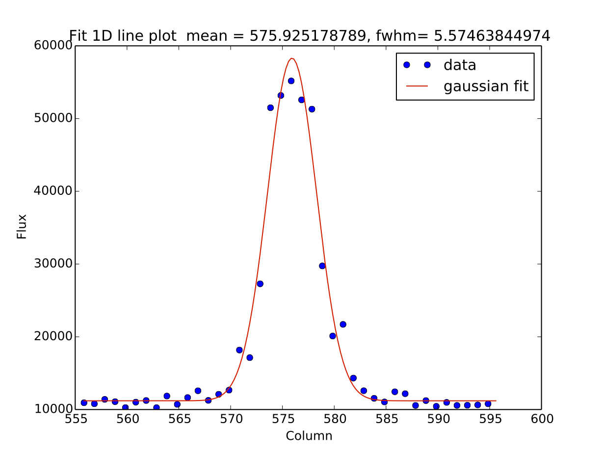
imexam prints the fit information to the screen
xc=585.660034       yc=697.499370
(585,697) mean=585.900, fwhm=5.653
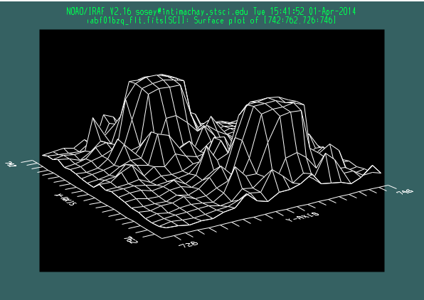
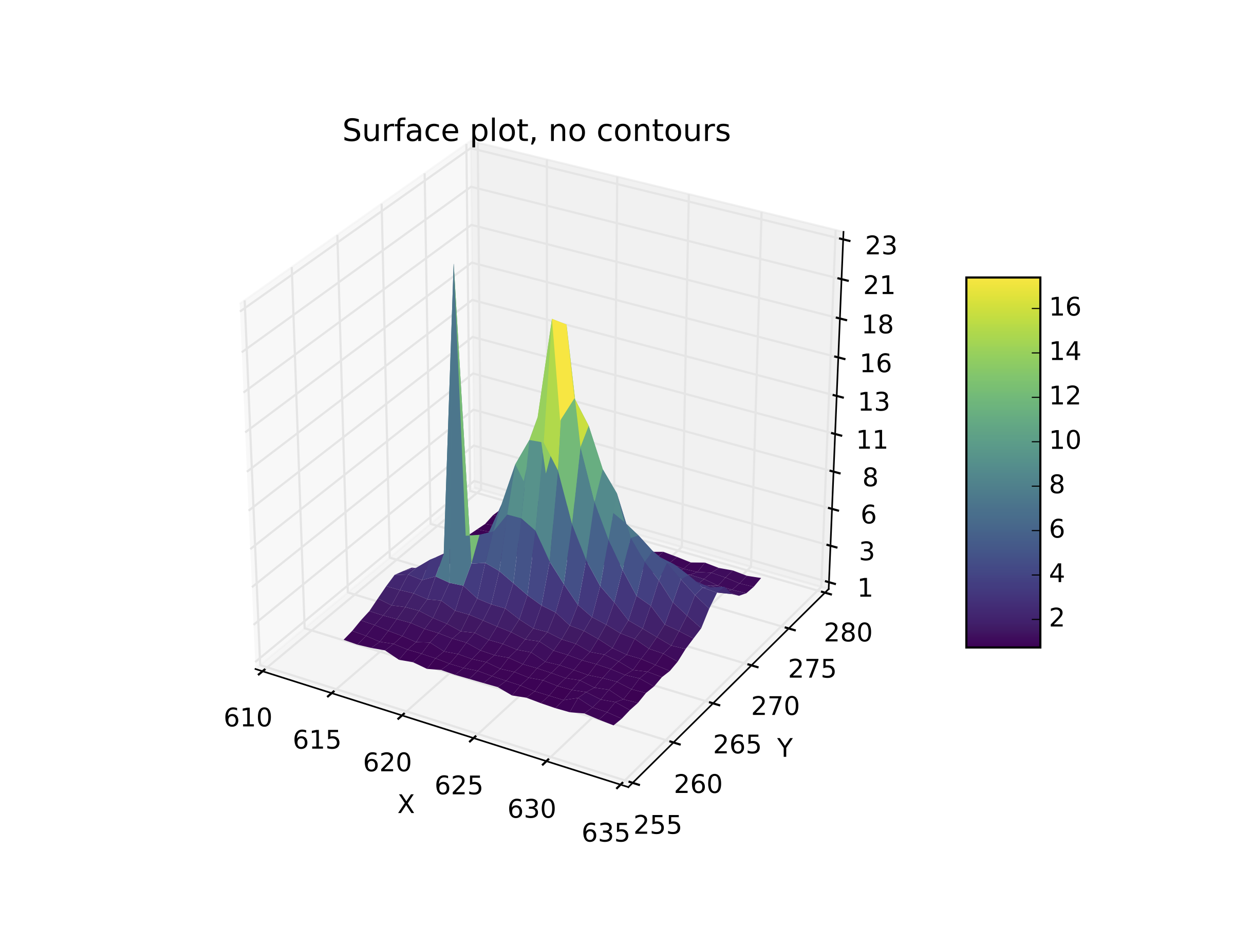
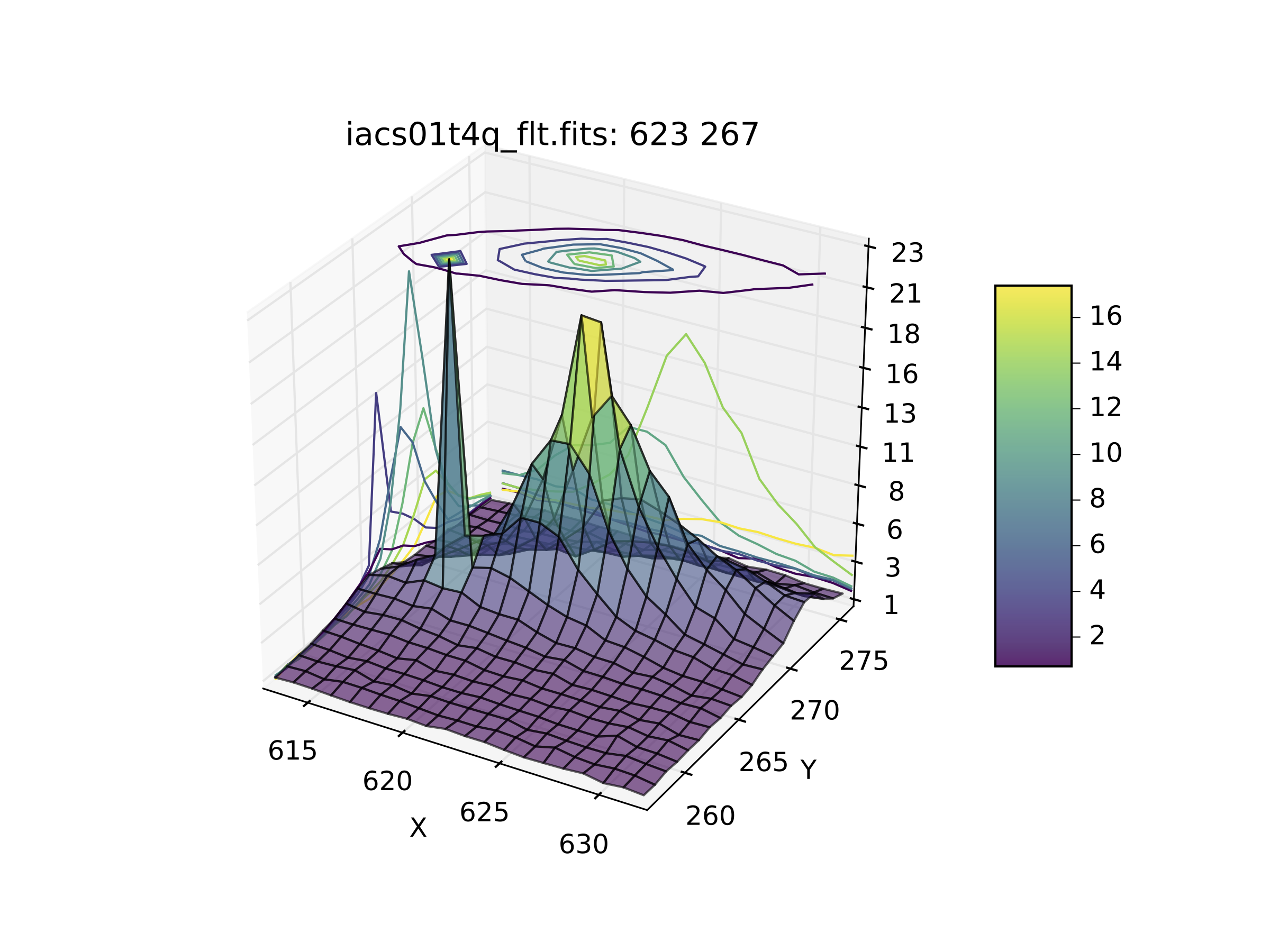
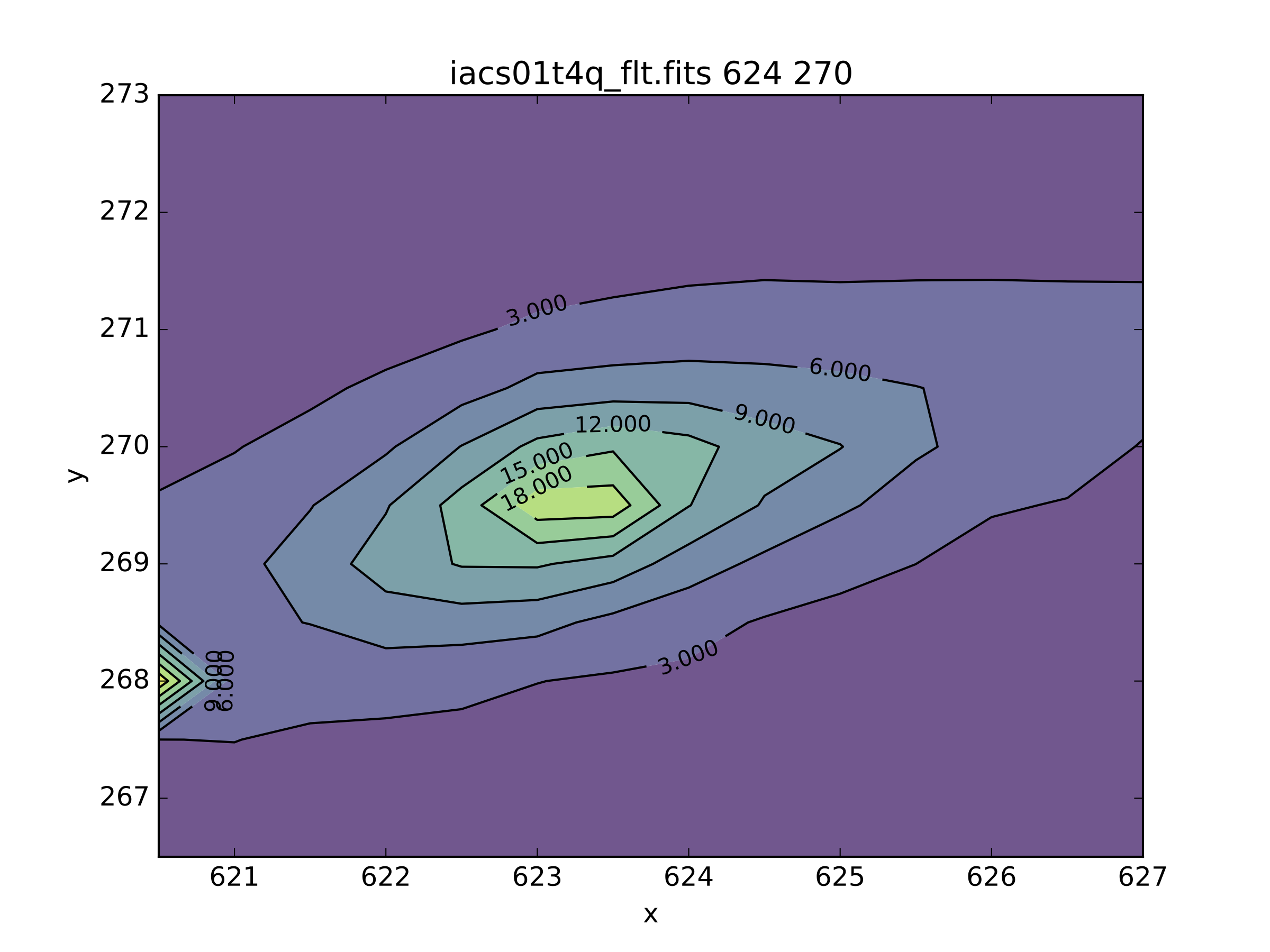
Surface plots
The default viewing angle for this package was set to that the axis are easiest to read, the user may choose a different azimuthal value as well.
The most fancy imexam surface plot is displayed, the user can alter it with the available options.