The imexam() method
This is the main method which allows live interaction with the image display when you are viewing your image or data array. If you execute imexam() while using the Ginga widget, it will display the available options, however they are always available for use via keystroke and are event-driven (using the same keys described below). In order to turn the key-press capture on and off while you have your mouse in the Ginga widget press the “i” key. Either the “i” or “q” key can be used to quit out of the examination mode.
- imexam ():
access realtime imexamine functions through the keyboard and mouse
Current recognized keys available during imexam are:
2 Make the next plot in a new window
a Aperture sum, with radius region_size
b Return the 2D gauss fit center of the object
c Return column plot
d Return the Center of Mass fit center of the object
e Return a contour plot in a region around the cursor
g Return curve of growth plot
h Return a histogram in the region around the cursor
j 1D [Gaussian1D default] line fit
k 1D [Gaussian1D default] column fit
l Return line plot
m Square region stats, in [region_size],default is median
r Return the radial profile plot
s Save current figure to disk as [plot_name]
t Make a fits image cutout using pointer location
w Display a surface plot around the cursor location
x Return x,y,value of pixel
y Return x,y,value of pixel


 aimexam(): return a dict of current parameters for aperture photometery

 cimexam(): return dict of current parameters for column plots

 dimexam(): return the center of mass around the current position

 eimexam(): return dict of current parameters for contour plots

 himexam(): return dict current parameters for histogram plots

 jimexam(): return dict current parameters for 1D line plots

 kimexam(): return dict of current parameters for 1D column plots

 limexam(): return dict of current parameters for  line plots

 gimexam(): return dict of current parameters for curve of growth plots

 rimexam(): return the dict of current parameters for radial profile plots

 wimexam(): return dict of current parameters for surface plots

 mimexam(): return dict of current parameters for area statistics

 timexam(): return a dict of the current parameters for image cutouts
Note
Some of the plots accept a marker type, any valid Matplotlib marker may be specified. See this page for the full list: http://matplotlib.org/api/markers_api.html#module-matplotlib.markers
The imexam key dictionary is stored inside the user object as <object_name>.exam.imexam_option_funcs{}. Each key in the dictionary is the keyboard key to recognize from the user, it’s associated value is a tuple which contains the name of the function to call and a description of what that function does. “q” is always assumed to be the returned key when the user wishes to quit interaction with the window. Users may change the default settings for each of the imexamine recognized keys by editing the associated dictionary. You can edit it directly, by accessing each of the values by their keyname and then reset mydict to values you prefer. You can also create a new dictionary of function which maps to your own
However, you can access the same dictionary and customize the plotting parameters using set_plot_pars. In the following example, I’m setting three of the parameters for the contour map, whose imexam key is “e”:
#customize the plotting parameters (or any function in the imexam loop)
viewer.set_plot_pars('e','title','This is my favorite galaxy')
viewer.set_plot_pars('e','ncontours',4)
viewer.set_plot_pars('e','cmap','YlOrRd') #see http://matplotlib.org/users/colormaps.html
where the full dictionary of available values can be found using the eimexam() function described above.:
In [1]: viewer.eimexam()
Out[2]:
{'ceiling': [None, 'Maximum value to be contoured'],
 'cmap': ['RdBu', 'Colormap (matplotlib style) for image'],
 'floor': [None, 'Minimum value to be contoured'],
 'function': ['contour'],
 'label': [True, 'Label major contours with their values? [bool]'],
 'linestyle': ['--', 'matplotlib linestyle'],
 'ncolumns': [15, 'Number of columns'],
 'ncontours': [8, 'Number of contours to be drawn'],
 'nlines': [15, 'Number of lines'],
 'title': [None, 'Title of the plot'],
 'xlabel': ['x', 'The string for the xaxis label'],
 'ylabel': ['y', 'The string for the yaxis label']}
Users may also add their own imexam keys and associated functions by registering them with the register(user_funct=dict()) method. The new binding will be added to the dictionary of imexamine functions as long as the key is unique. The new functions do not have to have default dictionaries association with them, but users are free to create them.
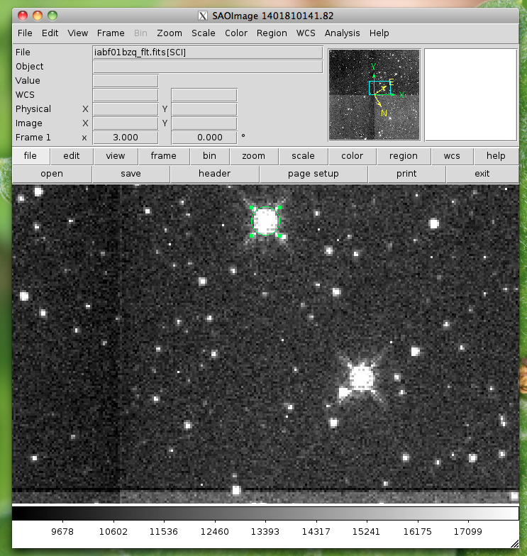
For all the examples below I will use a session similar to the following example:
#This will default to DS9 for the viewer

import imexam
viewer=imexam.connect()
viewer.load_fits('iabf01bzq_flt.fits')
viewer.scale()
viewer.panto_image(576,633)
viewer.zoom(3)
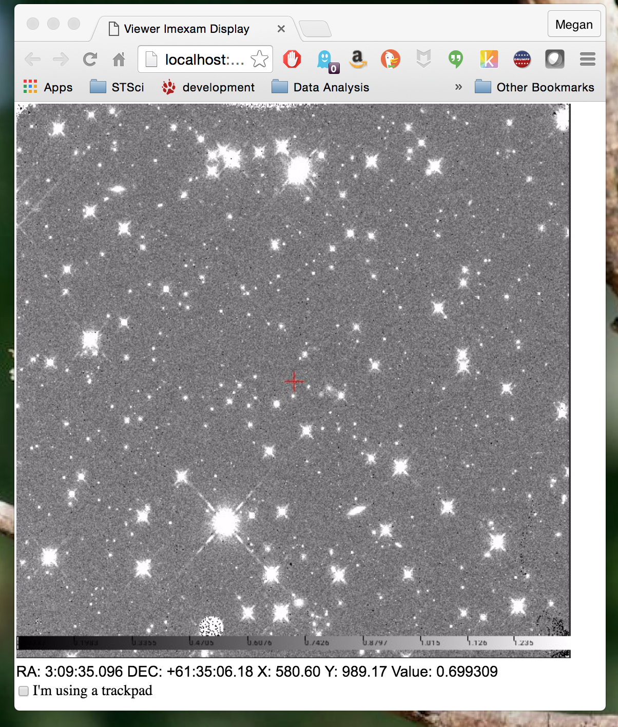
This will use Ginga (instead of the default DS9) for the viewer:
#Use Ginga for the image viewer, make sure it is installed

import imexam
viewer=imexam.connect(viewer='ginga')
viewer.load_fits('iabf01bzq_flt.fits')
viewer.scale()
viewer.panto_image(576,633)
viewer.zoom(3)
Circular Apterture Photometry
Aperture photometry is performed when you press the “a” key. It is implemented using the photutils python package, an affiliated package of astropy that is still in development.
Currently, the calculation which is performed is similar to the “,” or “a” IRAF imexamine keys. It is circular aperture photometry, centered on the mouse location at the time the key is pressed, with a background annulus subtraction for the sky. The radius of the aperture is set with the region_size keyword (default to 5 pixels). The annulus size is also set to the width, and taken a distance of skyrad pixels from the center. The pixels used to calculate the enclosed flux are those whose centers fall inside the radius distance, in the same way that IRAF imexamine computes the flux.
If center is set to True, and center_com is set to False, then a 2D Gaussian profile will be
used to refine the center of the object. If center_com is set to True, then a center of mass will
instead be calculated, using the delta box size around the object.
These are the default parameters for aperture photometry. They live in a dictionary in the exam object:
The direct access:

viewer.exam.aper_phot_pars= {'function':["aperphot",],
                'center': [True, "Center the object (choose center_type)"],
                'center_com': [False, "gaussian2d, True=center of mass"],
                'width':[5,"Width of sky annulus in pixels"],
                'subsky':[True,"Subtract a sky background?"],
                'skyrad':[15,"Distance to start sky annulus is pixels"],
                'radius':[5,"Radius of aperture for star flux"],
                'zmag':[25.,"zeropoint for the magnitude calculation"],
                'title': [None, 'Title of the plot'],
                'scale': ['zscale', 'How to scale the image'],
                'color_min': [None, 'Minimum color value'],
                'color_max': [None, 'Maximum color value'],
                'cmap': ['Greys', 'Matplotlib colormap to use'],
                'delta': [10, "bounding box for centering measurement"],
                }
Using the convenience function:

In [1]: viewer.aimexam()
Out[2]:
{'center': [True, "Center the object (choose center_type)"],
 'center_com': [False, "gaussian2d, True=center of mass"],
 'function': ['aper_phot'],
 'radius': [5, 'Radius of aperture for star flux'],
 'skyrad': [15, 'Distance to start sky annulus is pixels'],
 'subsky': [True, 'Subtract a sky background?'],
 'width': [5, 'Width of sky annulus in pixels'],
 'zmag': [25.0, 'zeropoint for the magnitude calculation'],
 'genplot': [True, 'Plot the apertures'],
 'title': [None, 'Title of the plot'],
 'scale': ['zscale', 'How to scale the image'],
 'color_min': [None, 'Minimum color value'],
 'color_max': [None, 'Maximum color value'],
 'cmap': ['Greys', 'Matplotlib colormap to use'],
 'delta': [10, "bounding box for centering measurement"]}
In order to change the width of the photometry aperture around the object you would do this::
viewer.set_plot_pars('a',"radius",10)
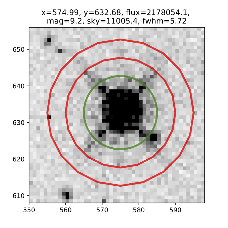
This is what the return looks like when you do photometry, where I’ve asked for photometry from the star above:
viewer.imexam()

xc=574.988523   yc=632.680333
x              y              radius         flux           mag(zpt=25.00) sky/pix        fwhm(pix)
574.99         632.68         10             2178054.09     9.15           11005.40       5.72
xc = xcenter, yc=ycenter; these were found using a Gaussian2D fit centered on the pixel location of the mouse. You can turn the fit off by setting the “center” parameter to “False”.
This is the resulting plot:
Using the Center of Mass:
com_center_pars = {"function": ["com_center",],
                   "delta": [10, "bounding box size"],
                   "oversample": [1., "oversample pixels by"],
                   }
Available 1D profiles
These include Gaussian1D, Moffat1D, MexicanHat1D, AiryDisk2D, and Polynomial1D.
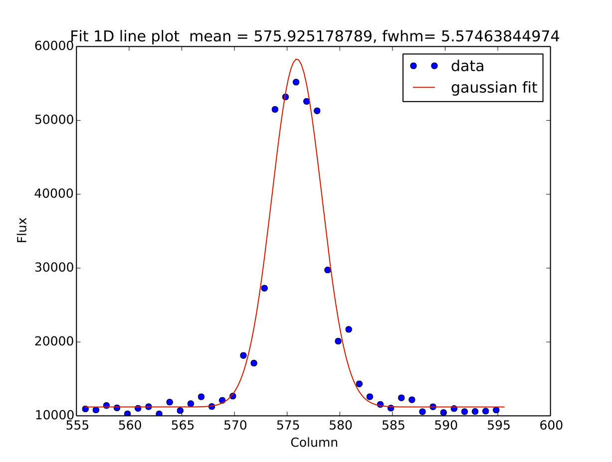
If you press the “j” or “k” keys, a 1D profile is fit to the data in either the line or column of the current pointer location. An option to use a Polynomial1D fit is also available, although not something of use for looking at stellar profiles. A plot of both the data and the fit + parameters is displayed. If the centering option is True, then the center of the flux is computed by fitting a 2d Gaussian to the data.
line_fit_pars={"function":["line_fit",],
               "func":["gaussian"," function for fitting [see available]"],
               "title":["Fit 1D line plot","Title of the plot"],
               "xlabel":["Line", "The string for the xaxis label"],
               "ylabel":["Flux", "The string for the yaxis label"],
               "background":[False, "Solve for background? [bool]"],
               "width":[10.0, "Background  width in pixels"],
               "xorder":[0, "Background terms to fit, 0=median"],
               "rplot":[20., "Plotting radius in pixels"],
               "pointmode":[True, "plot points instead of lines? [bool]"],
               "logx":[False, "log scale x-axis?"],
               "logy":[False, "log scale y-axis?"],
               "center":[True, "Recenter around the local max"],
               }
The column fit parameters are similar:
column_fit_pars={"function":["column_fit",],
                 "func":["Gaussian1D", "function for fitting [see available]"],
                 "title":["Fit 1D column plot", "Title of the plot"],
                 "xlabel":["Column", "The string for the xaxis label"],
                 "ylabel":["Flux", "The string for the yaxis label"],
                 "background":[False, "Solve for background? [bool]"],
                 "width":[10.0, "Background  width in pixels"],
                 "xorder":[0, "Background terms to fit, 0=median"],
                 "rplot":[20., "Plo tting radius in pixels"],
                 "pointmode":[True,"plot points instead of lines? [bool]"],
                 "logx":[False, "log scale x-axis?"],
                 "logy":[False, "log scale y-axis?"],
                 "center":[True, "Recenter around the local max"],
                 }
This is the resulting line fit:
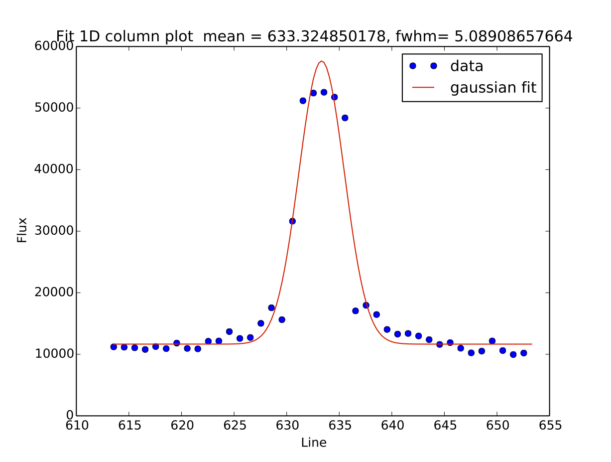
and the corresponding column fit:
Square region statistics
If you press the “m” key, the pixel values around the pointer location are calculated inside a box which has a side equal to the region_size, defaulted to 5 pixels, and using the statistical function chosen.
The user can map the function to any reasonable numpy function, it’s set to numpy.median by default:
report_stat_pars= {"function":["report_stat",],
                    "stat":["median", "numpy stat name or describe for scipy.stats"],
                    "region_size":[5, "region size in pixels to use"],
                }


[573:578,629:634] median: 50632.000000
You can change the statistic reported by changing the “stat” parameter:
viewer.set_plot_pars('m', "stat", "max")

[572:577,629:634] amax: 55271.000000
You can make a quick comparison of the max reported above with the line fit graph in the 1D gaussian profile example.
You can also choose to use the scipy.stats.describe function if you have scipy installed by changing the stat to “describe”; this will report the combined stats for the region::
pressed: m, report_stat
[551:556,653:658] describe:
nobs: 25
minamx: (0.51326549, 0.85604763)
mean 0.6851165890693665
variance: 0.00780616095289588
skew: 0.05719175934791565
kurtosis: -0.47930471400886976
Pixel Coordinates and Value
Hitting the ‘x’ or ‘y’ will return the x,y coordinate and pixel value under the mouse pointer.:
576.0 633.66667 55271.0
When not inside the imexam() loop, you can also set the location of the pointer using the wcs or pixel location you wish to view.
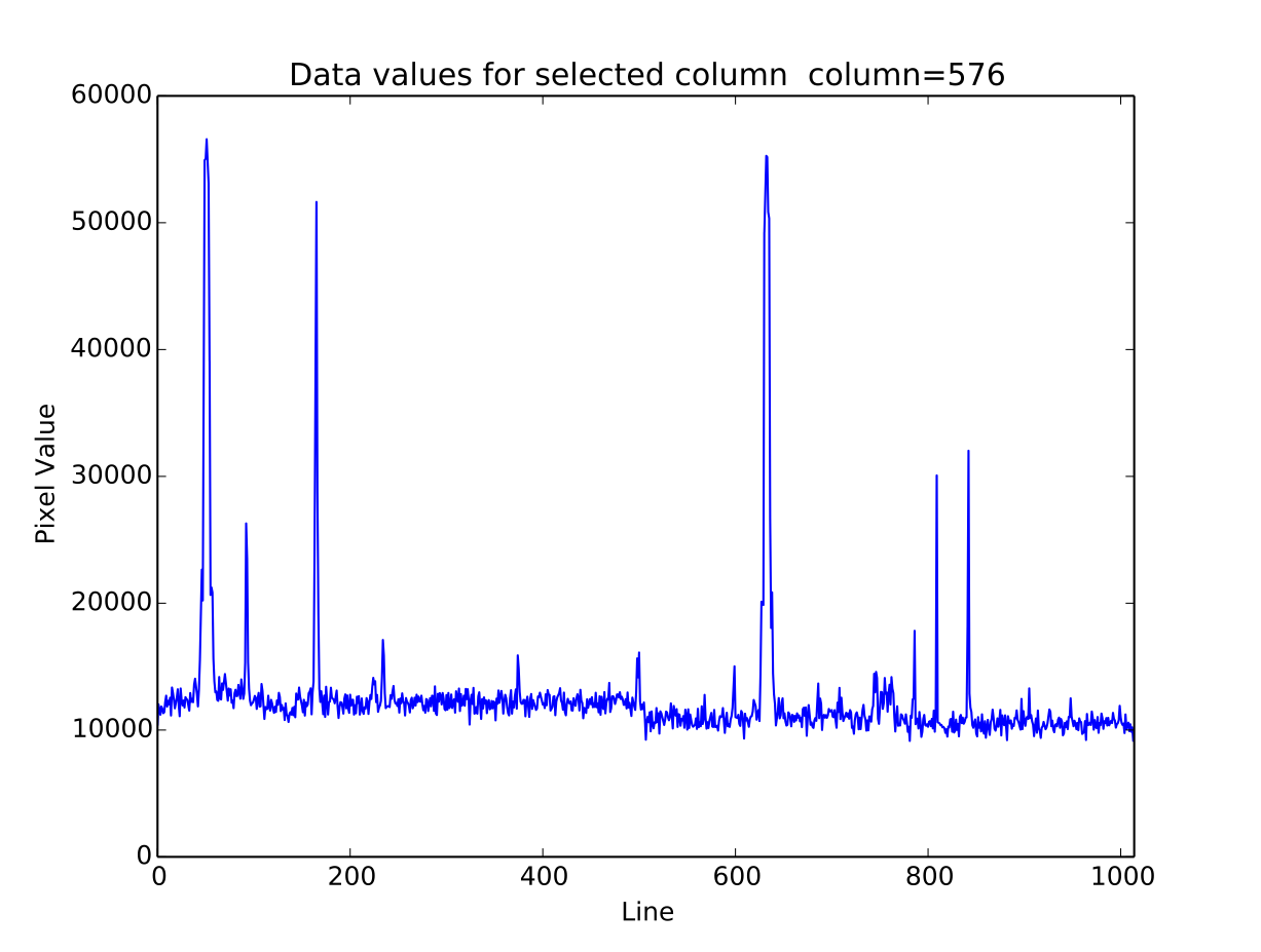
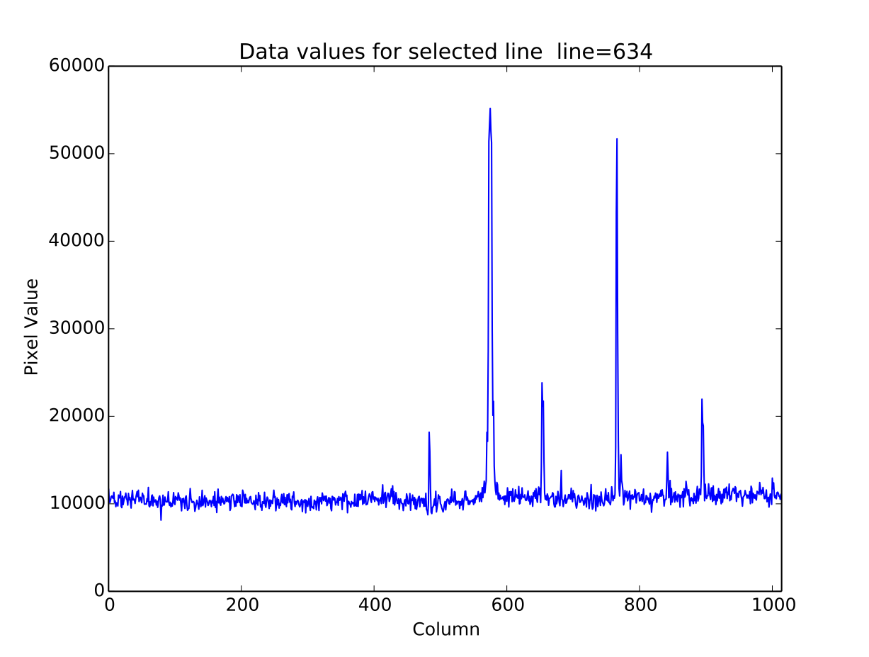
Line or Column plots
Pressing the “l” or “c” keys will display a plot of the points through either the line or column closest to the cursor location.
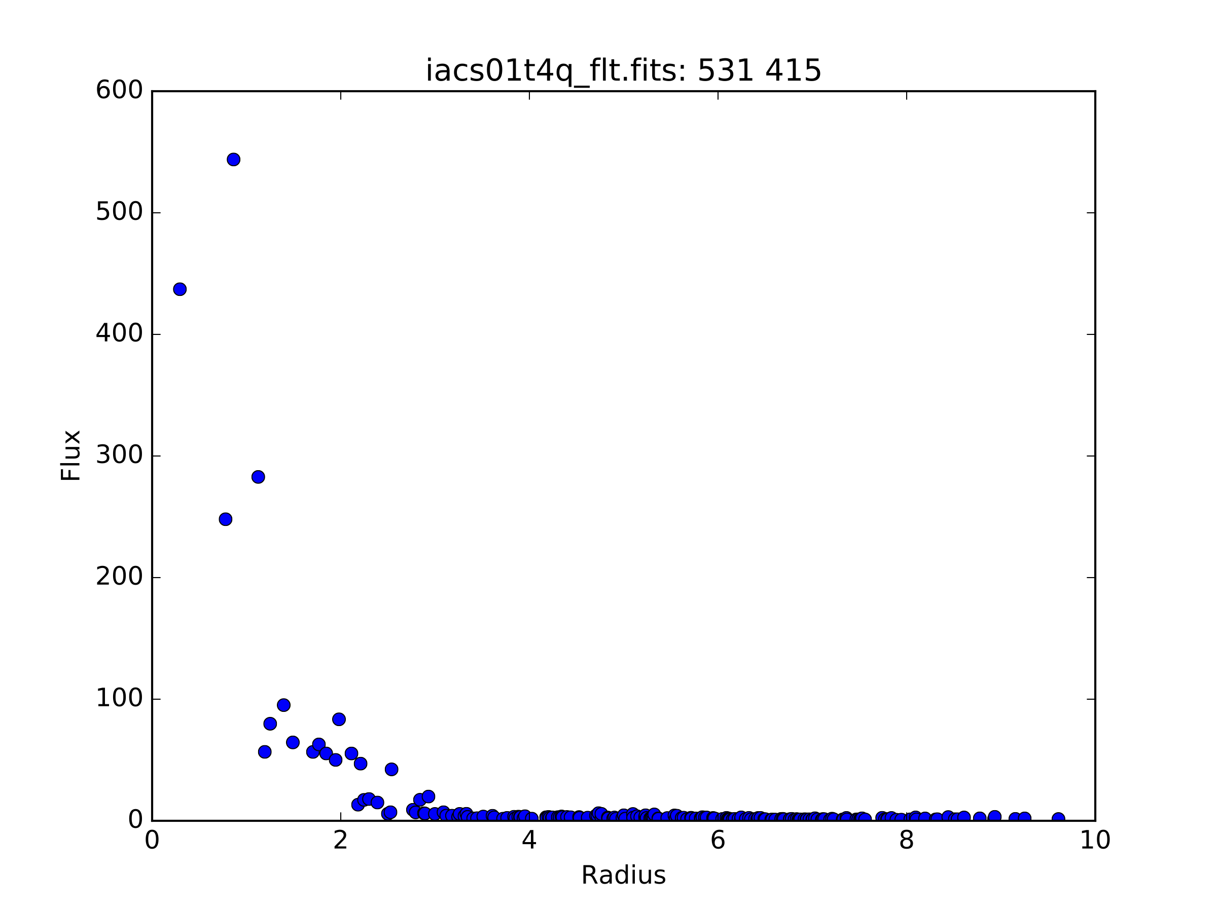
Radial Profile Plot
Pressing the “r” key displays a radial profile plot for the flux around the current pointer location. If centering is on, the center is computed close to the star using a Gaussian2D fit. The default plot uses every pixel
The available parameters are
radial_profile_pars = {"function": ["radial_profile_plot", ],
            "title": ["Radial Profile", "Title of the plot"],
            "xlabel": ["Radius", "The string for the xaxis label"],
            "ylabel": ["Summed Pixel Value", "The string for the yaxis label"],
            'pixels': [True, 'Plot all pixels at each radius? (False bins the data)']
            "fitplot": [False,"Overplot profile fit?"],
            "fittype":["Gaussian1D","Profile type to fit (gaussian)"],
            "center": [True, "Solve for center using 2d Gaussian? [bool]"],
            "background": [True, "Subtract background? [bool]"],
            "skyrad": [10., "Background inner radius in pixels, from center of object"],
            "width": [5., "Background annulus width in pixels"],
            "magzero": [25., "magnitude zero point"],
            "rplot": [8., "Plotting radius in pixels"],
            "pointmode": [True, "plot points instead of lines? [bool]"],
            "marker": ["o", "The marker character to use, matplotlib style"],
            "minflux": [0., "only measure flux above this value"],
            "getdata": [True, "return the plotted data values"]
            }
Radial profile plot for all pixels around the location:
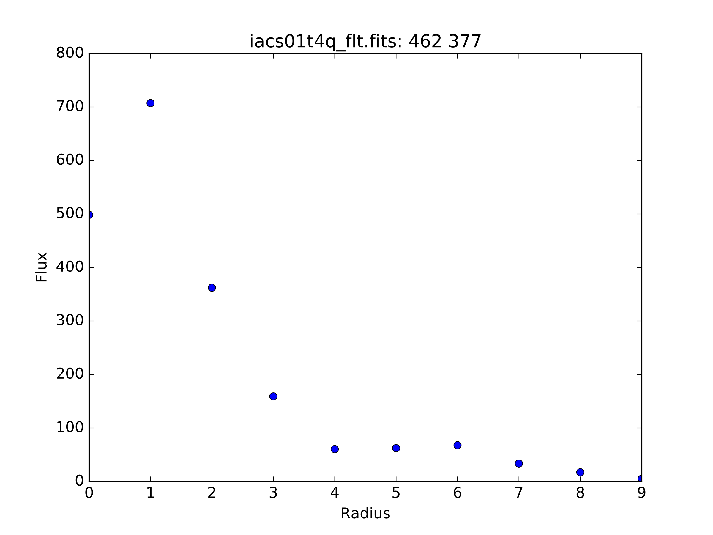
Radial profile plot for all pixels, binned to integer radii:
Curve of Growth plot
Pressing the “r” key displays a curve of growth for the flux around the current pointer location in successively larger radii. If centering is on, the center is computed close to the star using a 2d gaussian fit.
The available parameters are
curve_of_growth_pars={"function":["curve_of_growth_plot",],
                      "title":["Curve of Growth","Title of the plot"],
                      "xlabel":["radius","The string for the xaxis label"],
                      "ylabel":["Flux","The string for the yaxis label"],
                      "center":[True,"Solve for center using 2d Gaussian? [bool]"],
                      "background":[True,"Fit and subtract background? [bool]"],
                      "buffer":[25.,"Background inner radius in pixels,from center of star"],
                      "width":[5.,"Background annulus width in pixels"],
                      "magzero":[25.,"magnitude zero point"],
                      "rplot":[8.,"Plotting radius in pixels"],
                      "pointmode":[True,"plot points instead of lines? [bool]"],
                      "marker":["o","The marker character to use, matplotlib style"],
                      "logx":[False,"log scale x-axis?"],
                      "logy":[False,"log scale y-axis?"],
                      "minflux":[0., "only measure flux above this value"],
                      }
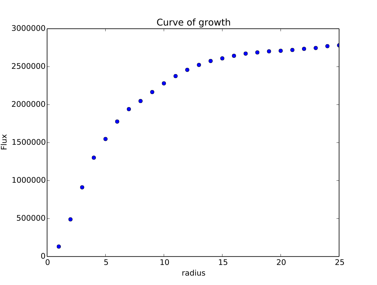
Returned to the screen is the data information from the plot, the (x,y) location of the center, followed by the radius and corresponding flux which was measured:
viewer.set_plot_pars('g',"rplot",25)  #set the default radius larger

xc=577.242311       yc=634.578361

at (x,y)=577,634
radii:[ 1  2  3  4  5  6  7  8  9 10 11 12 13 14 15 16 17 18 19 20 21 22 23 24 25]
flux:[131192.03694247041, 489485.48536408512, 911376.50226695999, 1301726.7189847208, 1547865.8684735354, 1777547.7859571185, 1940955.1267221647, 2047700.7156964755, 2165971.1952809561, 2280391.5901085823, 2376090.3555588746, 2458370.0006153183, 2523384.2243051622, 2575208.3657517368, 2609309.6524876151, 2643279.3635597304, 2672443.1546003688, 2687659.5178374872, 2702128.5513395425, 2709501.1520242952, 2720134.8632924128, 2734777.3482598308, 2746056.5231984705, 2770352.0070485324, 2781242.3299104609]
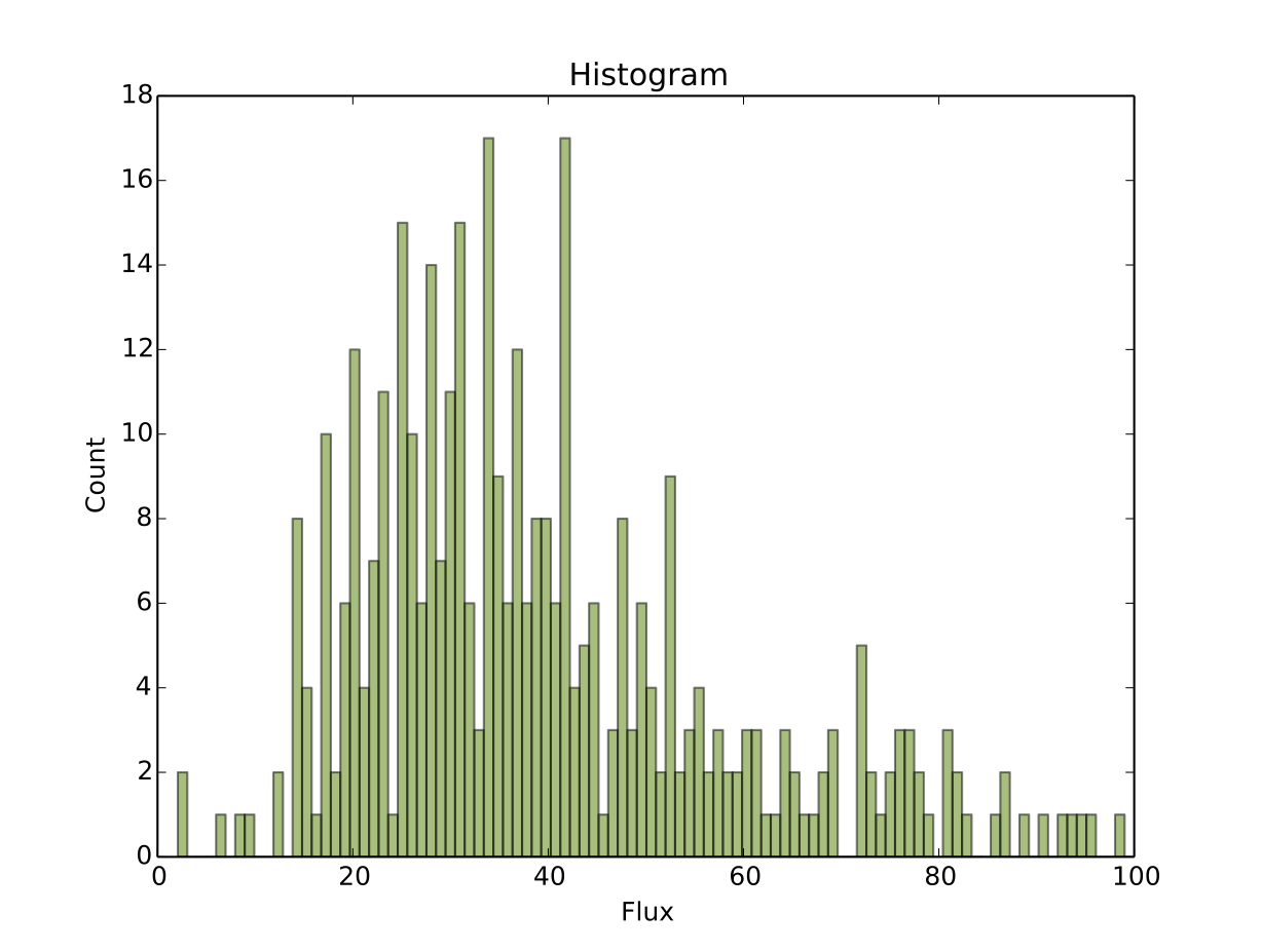
Histogram Plots
Pressing the “h” key will display a histogram of pixel values around the pixel location under the mouse pointer.
histogram_pars={"function":["histogram",],
                "title":["Histogram","Title of the plot"],
                "xlabel":["Flux (bin)","The string for the xaxis label"],
                "ylabel":["Count","The string for the yaxis label"],
                "ncolumns":[21,"Number of columns"],
                "nlines":[21,"Number of lines"],
                "nbins":[100,"Number of bins"],
                "z1":[None,"Minimum histogram intensity"],
                "z2":[100,"Maximum histogram intensity"],
                "pointmode":[True,"plot points instead of lines? [bool]"],
                "marker":["o","The marker character to use, matplotlib style"],
                "logx":[False,"log scale x-axis?"],
                "logy":[False,"log scale y-axis?"],
                }
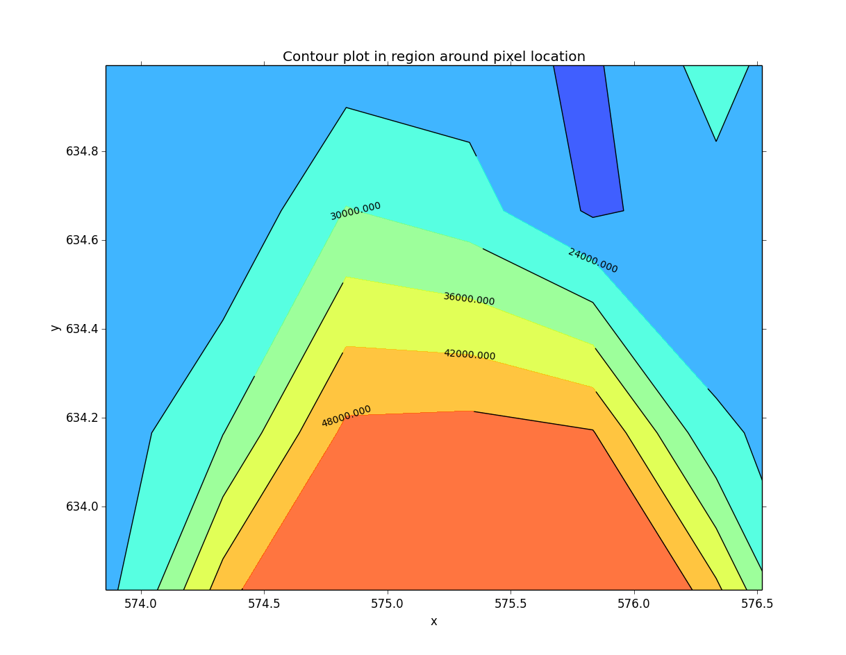
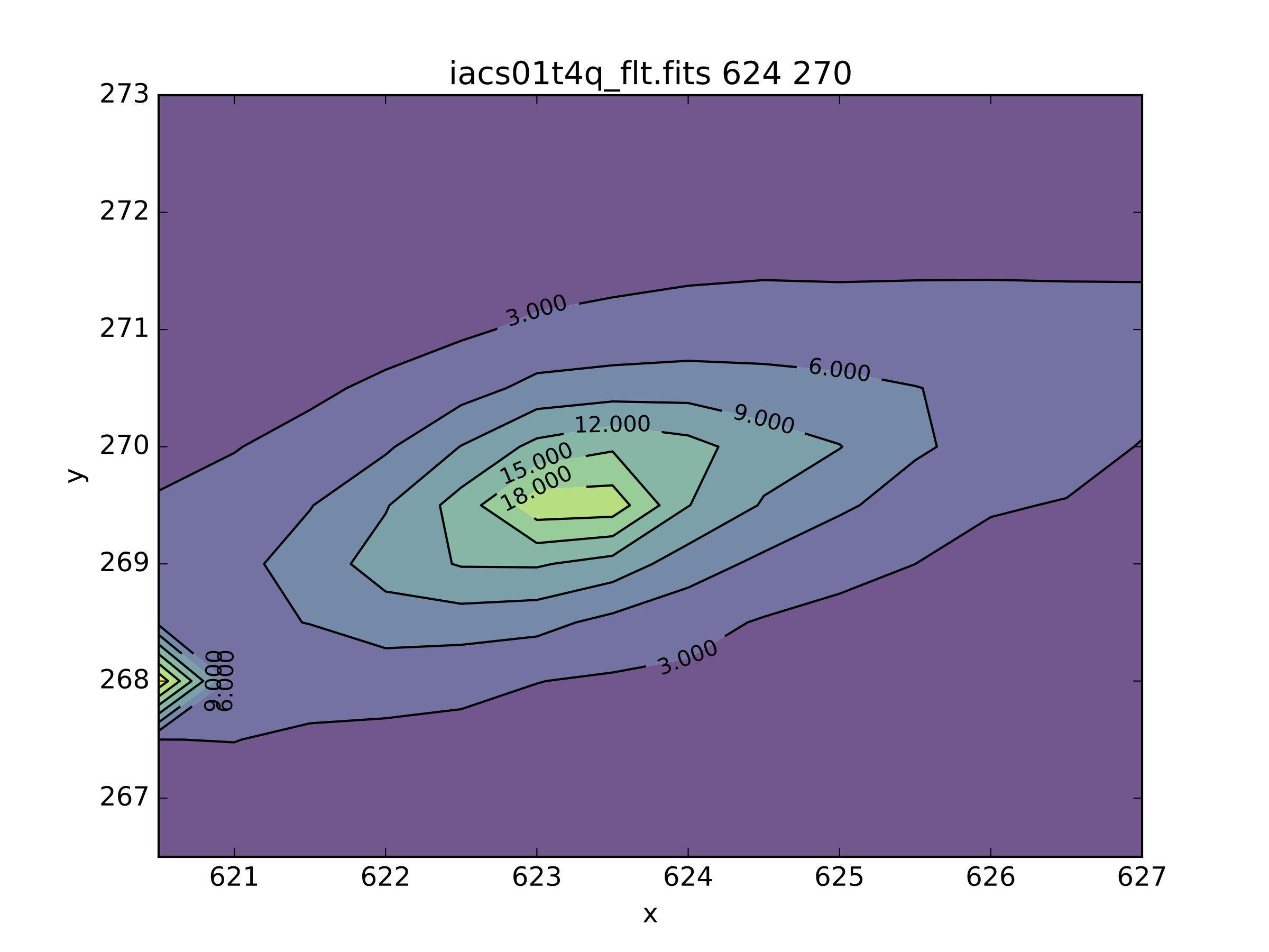
Contour Plots
Pressing the “e” key will display a contour plot around the clicked pixel location.
contour_pars={"function":["contour",],
                   "title":["Contour plot in region around pixel location","Title of the plot"],
                   "xlabel":["x","The string for the xaxis label"],
                   "ylabel":["y","The string for the yaxis label"],
                   "ncolumns":[15,"Number of columns"],
                   "nlines":[15,"Number of lines"],
                   "floor":[None,"Minimum value to be contoured"],
                   "ceiling":[None,"Maximum value to be contoured"],
                   "ncontours":[8,"Number of contours to be drawn"],
                   "linestyle":["--","matplotlib linestyle"],
                   "label":[True,"Label major contours with their values? [bool]"],
                   "cmap":["viridis","Colormap (matplotlib style) for image"],
                   }
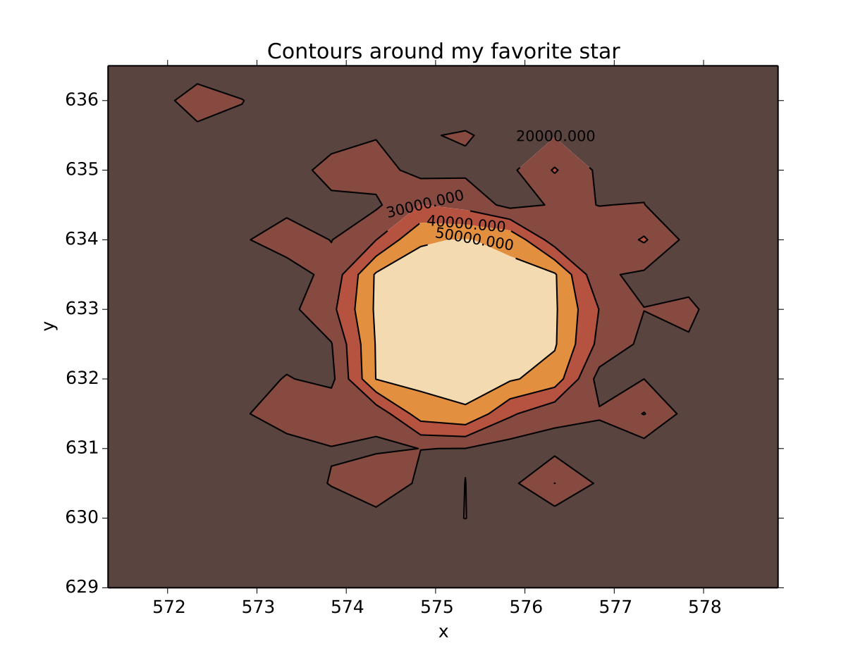
Here’s what it looks like if we change some of the default parameters:
viewer.set_plot_pars('e', "cmap", "gist_heat")
viewer.set_plot_pars('e', "title", "Contours around my favorite star")
viewer.set_plot_pars('e', "ncontours", 4)
viewer.set_plot_pars('e', "floor", 0)
Note
You can use any of the matplotlib standard cmaps, see the following link for more information: http://matplotlib.org/api/pyplot_summary.html?highlight=colormaps#matplotlib.pyplot.colormaps
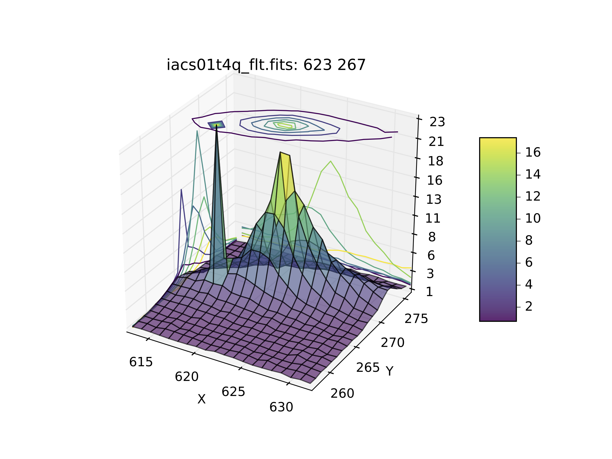
Surface Plots
Pressing the “s” key will display a 3D surface plot of pixel values around the mouse pointer location with the default parameters:
surface_pars = {"function": ["surface", ],
                "title": [None, "Title of the plot"],
                "xlabel": ["X", "The string for the xaxis label"],
                "ylabel": ["Y", "The string for the yaxis label"],
                "zlabel": [None, "Label for zaxis"],
                "ncolumns": [10, "Number of columns"],
                "nlines": [10, "Number of lines"],
                "azim": [None, "azimuthal viewing angle in degrees"],
                "floor": [None, "Minimum value to be contoured"],
                "ceiling": [None, "Maximum value to be contoured"],
                "stride": [1, "step size, higher vals will have less contour"],
                "cmap": ["viridis", "colormap (matplotlib) for display"],
                "fancy": [True, "This aint your grandpas iraf"],
                }
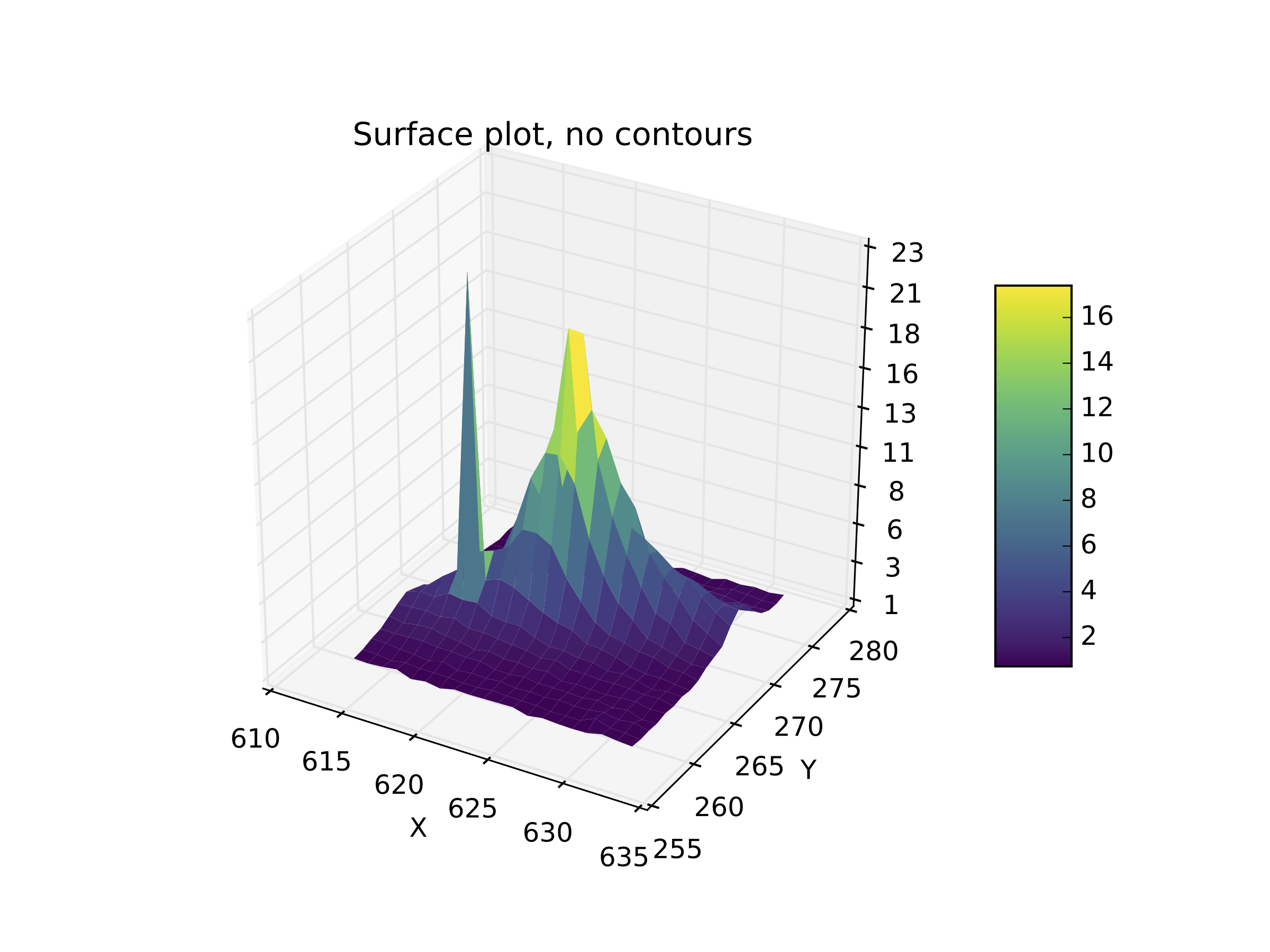
Or, with the contours turned off (by setting fancy to False) and changing the title:
Cutout a Simple FITS Image
Okay, I went to the star I like and pressed “t”. Let’s verify that we got what we wanted, it should be a cutout centered on the star that we’ve used in all the examples here:
image=fits.open('cutout_575.0_633.07fdinJ.fits')
viewer.frame(2)
viewer.view(image)
And the resulting frame view?
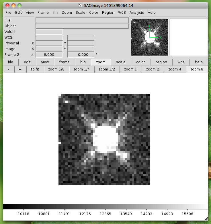
Sweet. Because this is a often used function I’ve made it a part of the standard selection set. If you wish to use the astropy 2D cutout method, you can create your own function which will also pass in the WCS object for the data so that the cutout retains it’s WCS information.
User Specified functions
Users may code their own functions and bind them to keys by registering them with the imexam dictionary through the register method that lives in the exam object. As long as a unique key is provided, the new binding will be added to the dictionary of imexamine functions. The new functions do not have to have default dictionaries associated with them. The binding is only good for the current object, new instantiations of imexam.connect() will not have the new function unless the user specifically registers them.
Here’s all the code for a function which saves the cursor location to a file called ‘test.list’ when the user presses the ‘p’ key:
def save_to_file(self,x,y,data):
    """Save the cursor location only to a file"""
    if data is None:
      data = self._data
    with open('test.list','a') as ofile:
      ofile.write("{0}\t{1}\n".format(x,y))
    print("Saved star to ",'test.list')
Now, import that into your python session, file, or here I’ll just copy paste the definition to the session. This is an important step because the function reference is what you are going to send to the registration method. The registration method wants you to supply a dictionary which contains the key you want to assign that function to during the imexam() loop, and a tuple with the function name and description:
my_dict = {'p': (save_to_file, 'Save cursor location to file')}

viewer.exam.register(my_dict)
User function: save_to_file added to imexam options with key p
Okay, so let’s try out our new function! We should be able to see it in the list of available options.
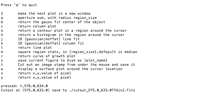
In [18]: a.imexam()

Press 'q' to quit

2       Make the next plot in a new window
a       Aperture sum, with radius region_size
b       Return the 2D gauss fit center of the object
c       Return column plot
e       Return a contour plot in a region around the cursor
g       Return curve of growth plot
h       Return a histogram in the region around the cursor
j       1D [Gaussian1D default] line fit
k       1D [Gaussian1D default] column fit
l       Return line plot
m       Square region stats, in [region_size],default is median
p       Save cursor location to file
r       Return the radial profile plot
s       Save current figure to disk as [plot_name]
t       Make a fits image cutout using pointer location
w       Display a surface plot around the cursor location
x       Return x,y,value of pixel
y       Return x,y,value of pixel

Current image /Users/sosey/test_images/iacs01t4q_flt.fits
pressed: p, save_to_file
Saved star to  test.list

In [19]: !more test.list
463.0   376.75
Plot Multiple Windows
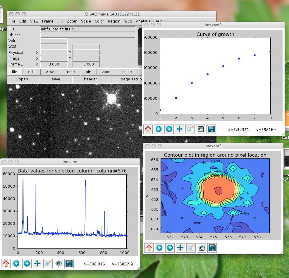
During a single viewer.imexam() session, you can choose to send your plots to multiple windows. Each window may only be used once, but if you would like to plot multiple things to compare, either the same plots for multiple objects or multiple types of plots for a single object, you can press the “2” key. This will save the current plotting window on your desktop and send the next plot to a new window. The plotting windows will be closed when you exit the imexam loop, so be sure to use the “s” key to save a quick copy of any plots you’d like to save for refernce. Here’s what that might look like:
#run aperture photometry("a"):

xc=576.522433       yc=634.578085
x              y              radius         flux           mag(zpt=25.00) sky            fwhm
576.52         634.58         5              1560462.68     9.52           10996.52       5.58

#make a column plot ("c")

#direct to a new window and make a contour plot ("e")
Plots now directed towards imexam2

#direct to a new window and make a curve of growth ("r")
Plots now directed towards imexam3

#the resulting curve of growth information on the screen
xc=576.855763       yc=634.911425

at (x,y)=576,634
radii:[1 2 3 4 5 6 7 8]
flux:[134294.19631173008, 521208.13904411002, 1017231.0442446949, 1297592.7076232315, 1568629.6771239617, 1813434.3810552177, 1935335.7549474821, 2049080.846300941]
This is what the workspace could look like with DS9 as the viewer:
As an aside, you can use the GUI tools on the bottom of the plot windows to move around the displayed data, such as zooming in and out, as shown below for the contour plot, which was also saved using the GUI save button: